Terminology
- Linear Models
- Linear Regression
- Regression modelling
- the General Linear Model includes:
- t-test
- ANOVA
- multivariate regression
We want to predict one thing (y) on the basis of another (x)
Terminology
- y: response, outcome, dependent variable
- x: predictor, covariate, independent variable
- used to help understand the variability in the response
Linear model
A function that describes a linear relationship between the response, \(y\), and the predictor, \(x\).
\[\begin{aligned} y &= \color{black}{\textbf{Model}} + \text{Error} \\[6pt]
&= \color{black}{\mathbf{f(\theta, x)}} + \epsilon \\[6pt]
&= \mathrm{intercept} + \mathrm{slope} \cdot x + \epsilon \\[6pt]
&= \alpha + \beta x + \epsilon \\[6pt]
\theta &= (\alpha, \beta) \\[6pt]
\end{aligned}\]
Linear model
A function that describes a linear relationship between the response, \(y\), and the predictor, \(x\).
\[\begin{aligned} y &= \color{black}{\textbf{Model}} + \text{Error} \\[6pt]
&= \color{black}{\mathbf{f(\theta, x)}} + \epsilon \\[6pt]
&= \mathrm{intercept} + \mathrm{slope} \cdot x + \epsilon \\[6pt]
&= \beta_0 + \beta_1 x + \epsilon \\[6pt]
\theta &= (\beta_0, \beta_1) \\[6pt]
\end{aligned}\]
Linear model
\[
\begin{aligned} y &= \color{purple}{\textbf{Model}} + \text{Error} \\[8pt]
&= \color{purple}{\mathbf{f(\theta, x)}} + \epsilon \\[8pt]
&= \color{purple}{\alpha + \beta x} + \epsilon \\[8pt]
\end{aligned}
\]
Linear model + residual error
\[\begin{aligned} y &= \color{purple}{\textbf{Model}} + \color{blue}{\textbf{Error}} \\[8pt]
&= \color{purple}{\mathbf{f(\theta, x)}} + \color{blue}{\boldsymbol{\epsilon}} \\[8pt]
&= \color{purple}{\alpha + \beta x} + \color{blue}{\boldsymbol{\epsilon}} \\[8pt]
\end{aligned}\]
Uses
- Prediction
- Extrapolation
- Associations / correlation
- Causal inference
Terminology
Regression slopes \(\beta\) are often referred to as effects
- e.g. \(\beta = 1.5\) is the numerical effect of \(x\) on \(y\) in the model
- but effect implies causality
- better called coefficient to be neutral
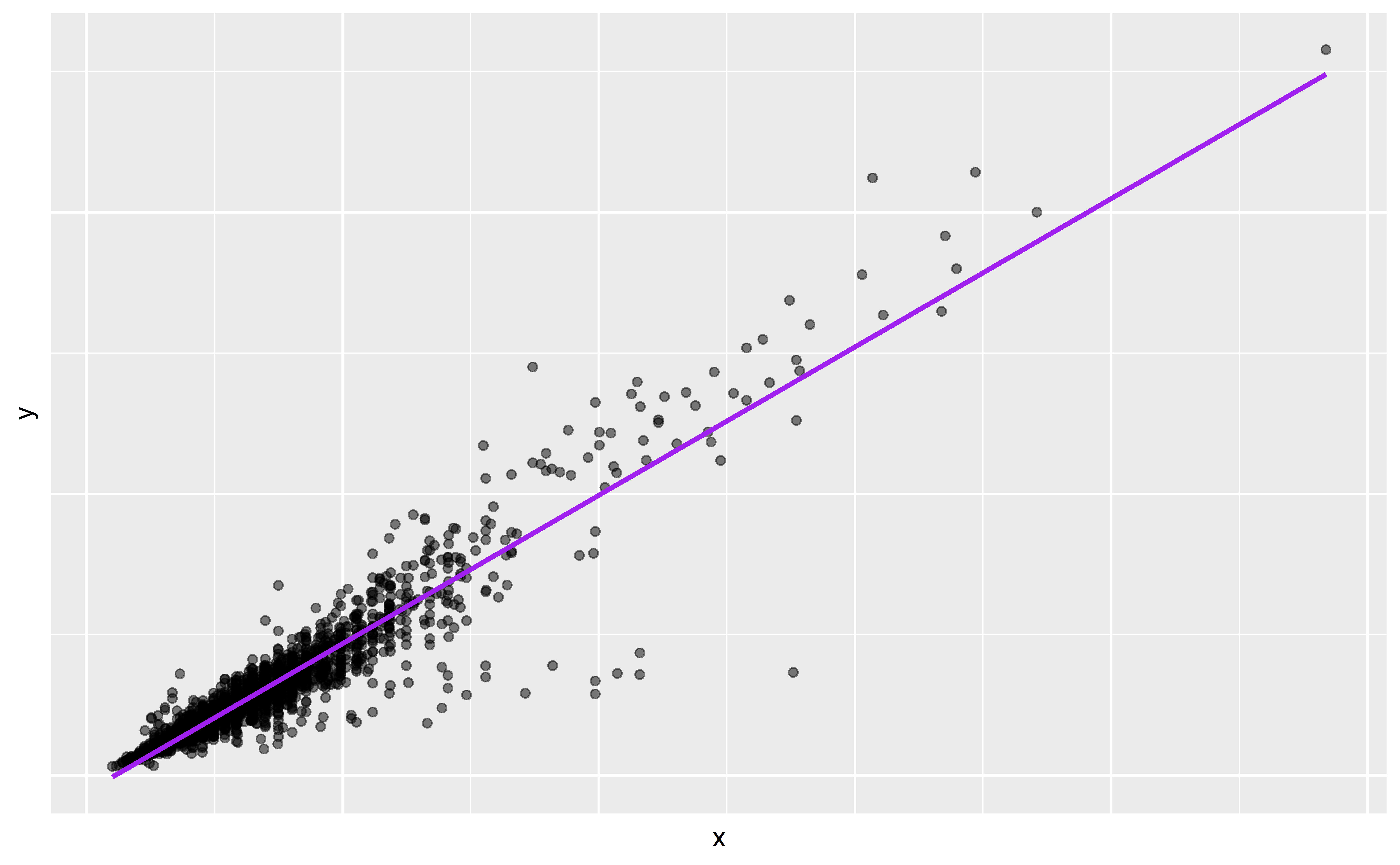
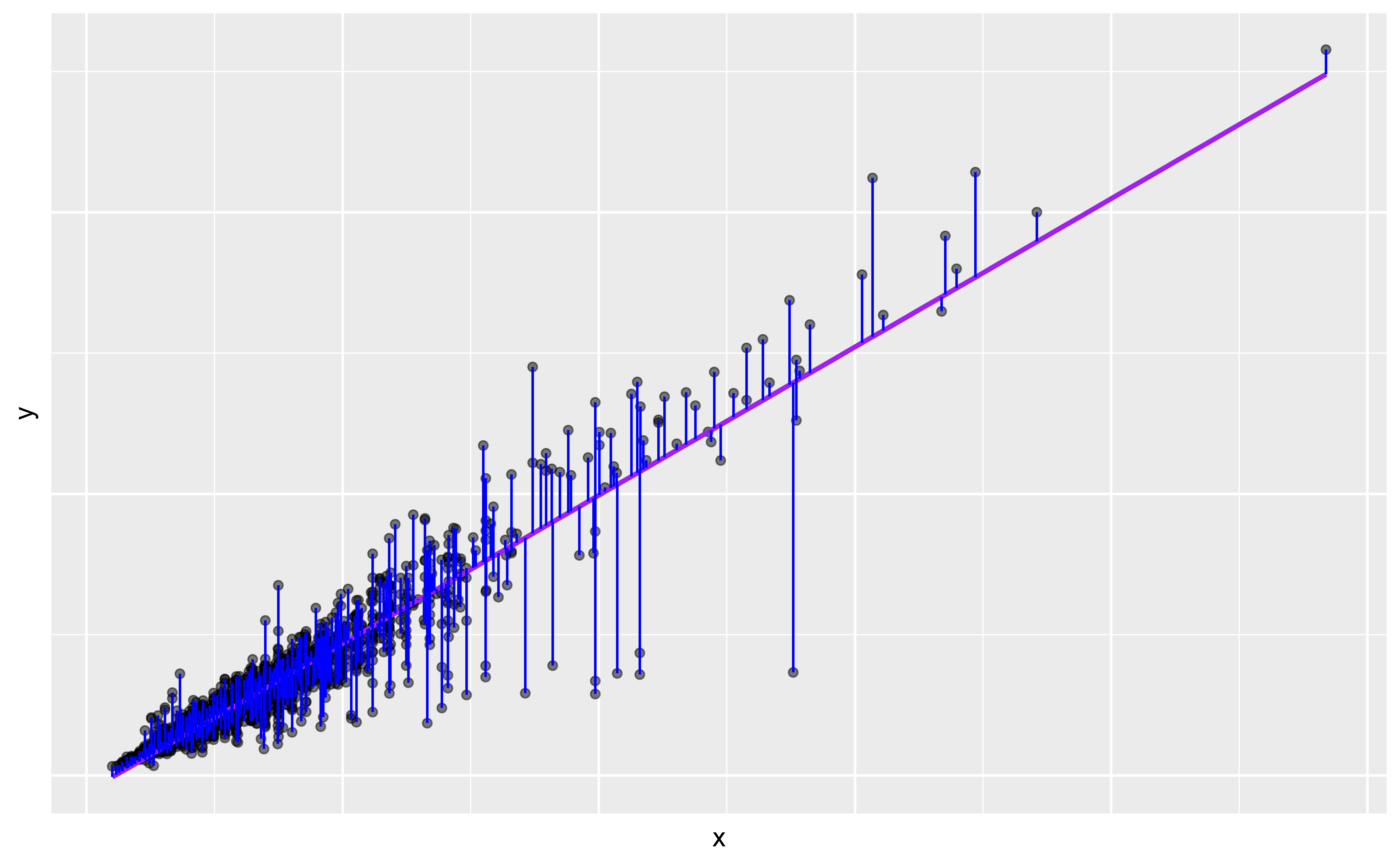
Frequentist linear regression
- find the best-fit line which minimises residuals
- point estimate for the relationship between x and y
- assume Gaussian approximation for confidence intervals
- test null hypothesis of zero slope \(\beta = 0\)
![]()
Bayesian linear regression
- find the (posterior) distribution of plausible relationships between x and y
- i.e. \(P(\theta | y) \propto P(\theta) P(y | \theta)\)
- use Bayes rule via MCMC
- no Gaussian assumption needed for parameters (only measurement error)
- hypothesis test is irrelevant - posterior \(\theta\) captures all information
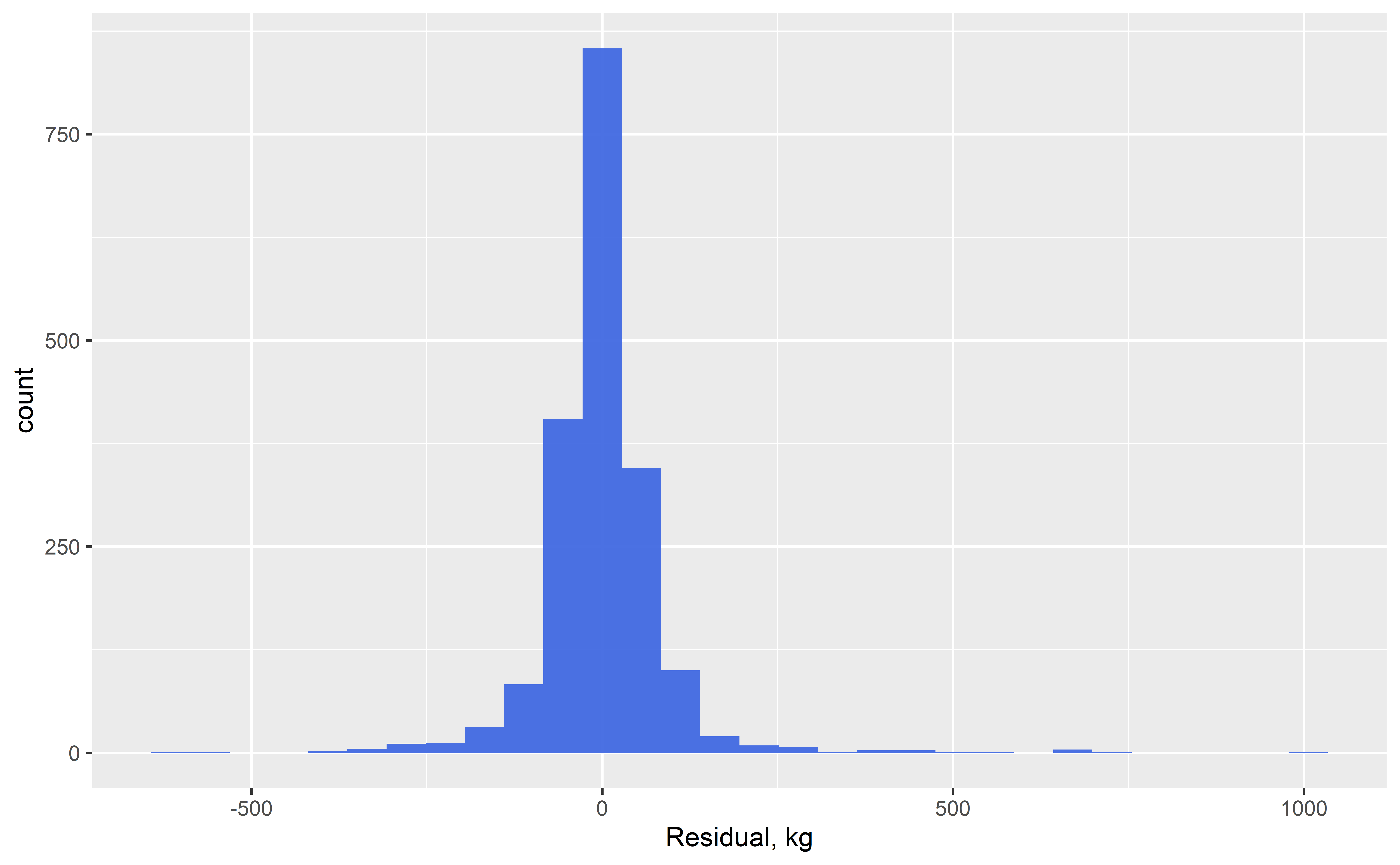
Assumptions
- Constant variance across the range in \(x\)
- 0 zero error in \(x\)
- Linearity
- Independent samples
- Normally-distributed measurement error
- mnemonic: C0LIN
Extensions to Linear Modelling
When assumptions are not met …
- Independent samples - hierarchical & mixed-effect models; spatial/time series
- Linearity - Generalised Linear Models; General Additive Models
- Normally-distributed measurement error - Generalised Linear Models
Theory into practice …
Two practicals
- Bayesian estimation of the parameters of linear models
- use package in R for MCMC
rstanarm
- easy syntax for specifying model
Consider:
- convergence checks
- model predictions
- prior distributions
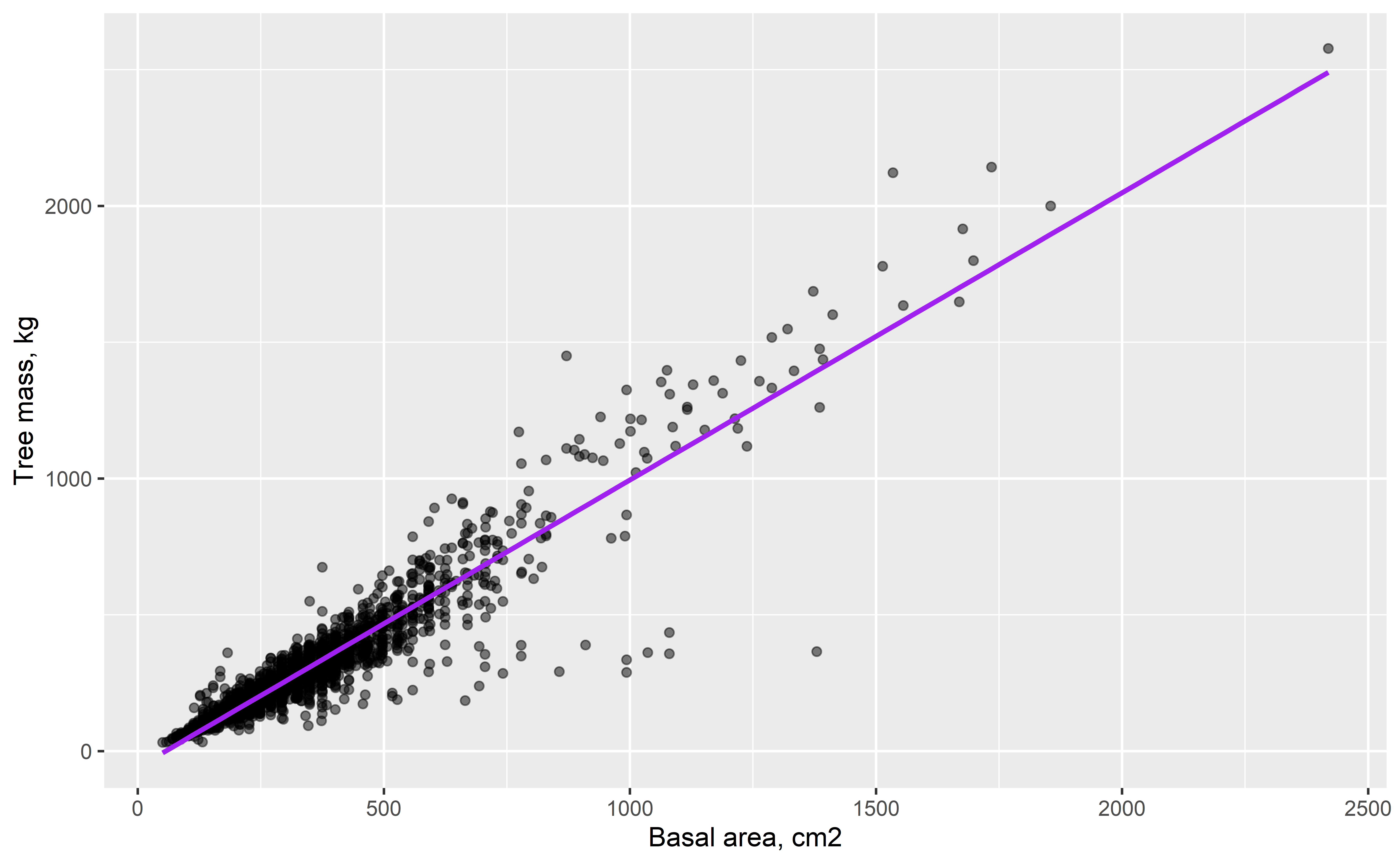
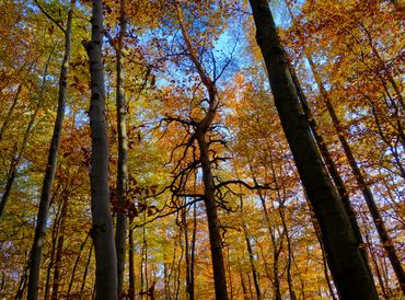
Tree allometry
- How does tree mass scale with stem diameter?
- Can we reliably estimate forest carbon stocks from simple measurements?
Tree allometry
- How does tree mass scale with stem diameter?
- Can we reliably estimate forest carbon stocks from simple measurements?
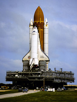
Space Shuttle Challenger
- How do we assess risks from uncertain linear relationships?
- How do we combine data with prior knowledge?
Syntax
m <- lm(tree_mass ~ basal_area, data = df)

m <- stan_glm(tree_mass ~ basal_area, data = df)