Bias Correction of Climate Model Output#
Paper (Chapter 4)
Notebook Repository
Method Repository
Ongoing Development
![]()
Primary Contact: Dr. Jeremy Carter | Notebook Top-to-Bottom Runtime ~ 2 Minutes
Physically based climate models are highly-multidimensional and computationally demanding. Simulation runs are often tuned for specific variables and typically observe a non-insignificant bias in other variables. Depending on what variables your specific research question focuses on it’s often desirable to perform postprocessing bias correction. In-situ measurements of variables can be used to help apply a bias correction. Where the in-situ measurements are sparse it’s important to consider uncertainty, depending on factors such as the underlying spatial covariance between points.
Gaussian processes are used to explicitly model spatial covariance between points and to estimate uncertainties when applying bias correction across the whole domain. A Bayesian hierarchical model is constructed to promote uncertainty propagation across the different components of the model.
Running the Notebook:
To run the notebook it is advised to first clone the repository housing the notebook (’git clone NERC-CEH/ds-toolbox-notebook-biascorrection.git’). This will create a folder in the current directory called ds-toolbox-notebook-biascorrection, which holds all the relevant files including the notebook, environment file and relevant input data. The next step is to create a conda environment with the right packages installed using the clean yml file (’conda env create -f environment-clean.yml’), which creates the jbook_BCA environment that can be activated using ‘conda activate jbook_BCA’. At this point the user can either run code from the notebook in their preferred IDE or via the jupyter interface using the command ‘jupyter notebook’. If using VSCode one recommended approach is to use Python interactive windows and copy and paste snippets of code to run from the notebook.
Data Access:
A partially pre-processed example input dataset is used in this tutorial for simplicity. Raw state-of-the-art climate model output for Antarctica can be accessed via the Antarctic CORDEX project and emailing the primary contacts listed. The automatic weather station data can be accessed via the AntAWS Dataset. The post-inference data for this notebook is available at Bias Correction Walkthrough Tutorial Inference Data and is retrieved in the Parameter Inference section.
Statistical Concepts:
Gaussian processes represent probability distributions over a function of values by considering the covariance between points. For example, consider some spatial surface of mean temperature over a region. The values will vary smoothly over the domain and so values of nearby points are spatially correlated. To interpolate across the surface and to express what the likelihood is of the particular surface of values observed you need to consider the spatial correlation. This is what Gaussian processes do by parameterising the covariance as a function of distance between points. Since Gaussian processes represent a probability distribution over the function you can estimate an expectation and also uncertainty in predictions.
Generalisability:
Gaussian processes are highly generalisable as they don’t assume a fixed functional form of the underlying process. That is many different types of spatial and/or temporal surfaces can be modelled adequately through them, including oscillatory functions for example. They are applicable across domains such as regression, classification, time-series modelling and spatial analysis. Gaussian processes are also highly interpretable and resistant to overfitting due to being defined by a limited number of hyper-parameters. Finally, providing a probabilistic approach, they also capture uncertainty in estimates, important for various real-world applications and data science pipelines leading to decision-making. The specific example in this notebook is generalisable to any scenario involving combining multiple spatio-temporal datasets, particularly when a good-coverage biased dataset is combined with a poor-coverage unbiased dataset.
Warning: Computational Demands
While the notebook runs top-to-bottom in <5mins this is achieved through loading in inference results. The method presented in this notebook is very computationally demanding even for small datasets and was developed with the idea of getting maximum utility out of the limited weather station data available over Antarctica. The methodology is still being worked on and if the reader is interested in contributing/raising issues this would be very welcomed via the repository link and issues tab.
It is suggested that the reader takes away some of the core concepts presented in the pipeline and utilises particular code snippets to apply to their specific area of application. The Bayesian modelling framework is highly-flexible and so specific modelling adaptions should be simple to incorporate.
Introduction#
This notebook demonstrates an approach to bias correction that utilises Gaussian Processes (GPs) and a Bayesian hierarchical framework. The method is applied to bias correcting temperature data from a climate model over Antarctica using in-situ observations from automatic weather stations. Since the weather stations are both spatially and temporally sparse it’s important to capture uncertainty in the correction. Further detail is available at: J.Carter Thesis (Chapter 4). The code is in ongoing development and is available at: Bias Correction Application. The datasets and modules needed to run this notebook are available via the jupterbook_render branch of the repository.
Importing Required Libraries and Loading Data#
The data for this tutorial is stored as NetCDF files. This is a common file format for climate model output and is handled well by the Xarray Python package, which can be thought of as a Pandas equivalent for efficient handling of multidimensional data. Xarray loads data as ‘datasets’ and ‘dataarrays’. The model in this tutorial is defined using the Python packages Numpyro and TinyGP, which are compatible. Numpyro provides an intuitive probabilistic programming language for Bayesian statistics, built ontop of JAX and with NumPy based syntax. TinyGP provides a lightweight and intuitive package for working with Gaussian Process objects.
# Loading Data
data_path = os.path.join(os.getcwd(),"data","")

ds_aws = xr.open_dataset(f'{data_path}ds_aws.nc') # Automatic Weather Station Data
ds_climate = xr.open_dataset(f'{data_path}ds_climate.nc') # Climate Model Data
Using Xarray datasets provides nice interactive tables of the multidimensional data:
# Displaying the AWS data
ds_aws
# Displaying the climate model data
ds_climate
# Computing basic summary statistics using the pandas port of xarray objects
print('Summary of Automatic Weather Station Data \n',
      ds_aws.to_dataframe().describe()[['elevation','latitude','temperature']])
print('\n Summary of Climate Model Data \n',
      ds_climate.to_dataframe().describe()[['elevation','latitude','temperature']])
Data Exploration#
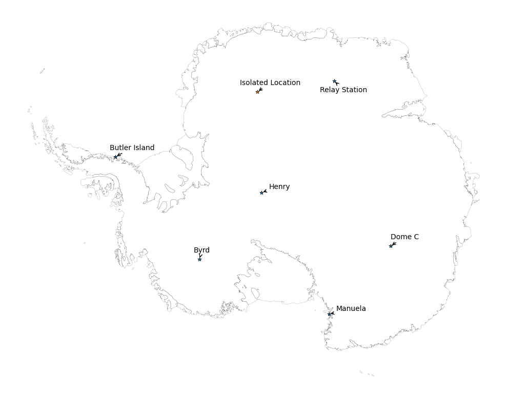
Initial data exploration is essential for informing our model construction. It includes examining the spatial and temporal distributions of the data and relationships between variables and potential predictors. To start we’ll examine the spatial distribution of weather stations, plotting over the grid of the climate model.
Spatial Distribution of Weather Stations#
Coordinate Systems:
Note that for plotting we use a specific rotated coordinate system (defined below). The ‘glon’ and ‘glat’ fields are in this coordinate system and it was created to get around issues assoicated with plotting the shapefile when the longitude flips between -180 to 180.
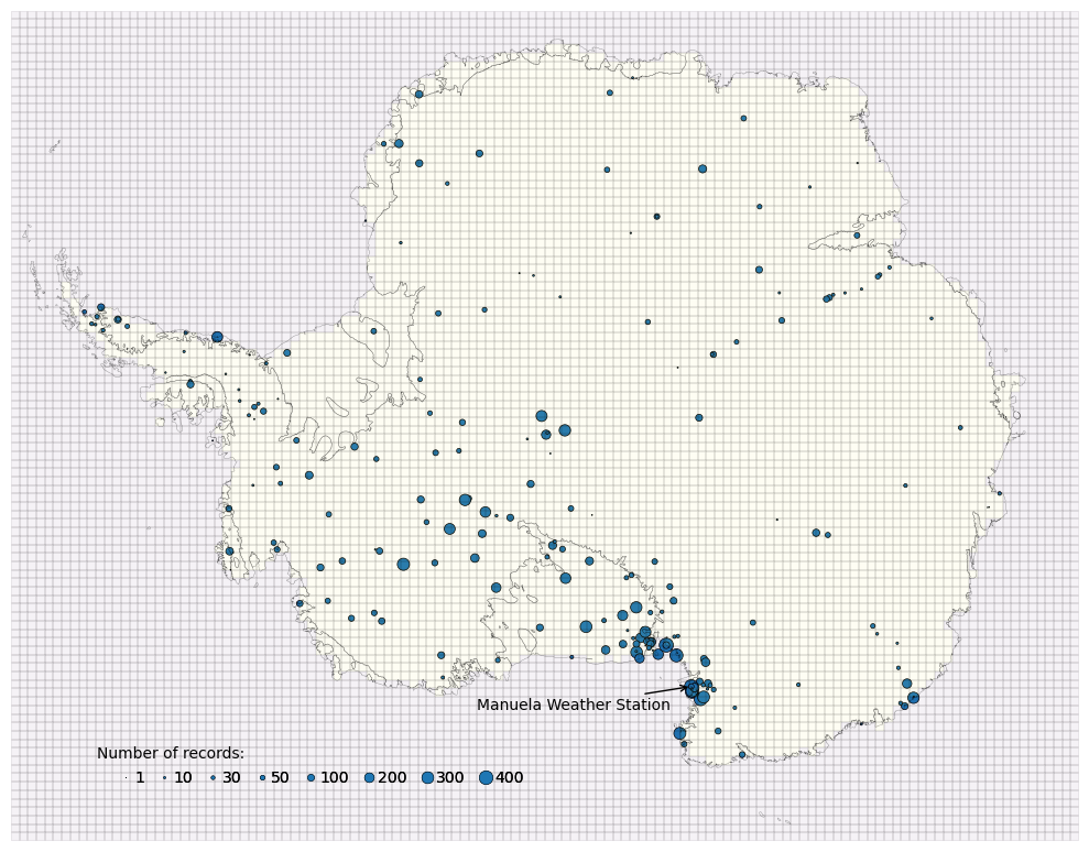
It is clear that the spatial distribution of weather stations is not uniform over the domain. There are certain regions containing high-density clusters of stations. This will induce a bias in the bias-correction itself when conducted over the whole domain, with corrections skewed towards these regions. If these clusters occurred randomly then modelling the spatial correlation between sites would be adequate to account for the distribution. Instead it is likely these regions were chosen for specific features, such as having anomalously high temperatures, which is difficult to account for in the model. We don’t directly attempt to solve this problem but it is noted as a remaining limitation.
Time Series and Distribution of Single Weather Station (Manuela)#
Comparisons are made between the time series for the Manuela weather station and the nearest grid-cell of the climate model output. The time series represents the average temperature for each month and the values are aggregated from hourly measurements of the raw data (preprocessed in this notebook for simplicity).
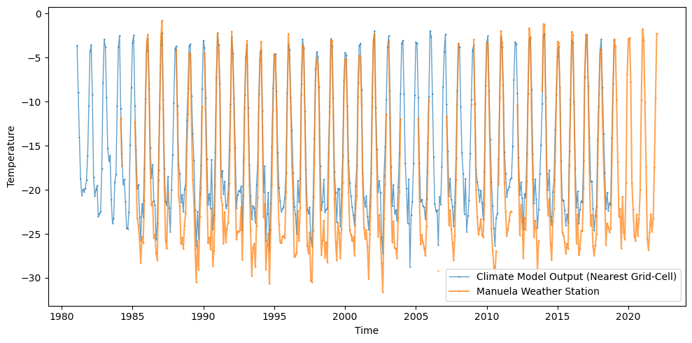
The Manuela weather station has one of the highest numbers of temperature records, spanning from 1984-2021. The time series for the climate model spans 1981-2019. It’s clear that the variance in the time series are dominated by the seasonal cycle and that any bias in for example the mean will have some seasonal dependency. The PDFs for the 2 time series are plot below.
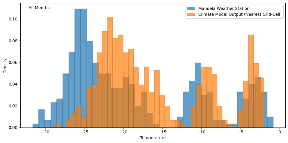
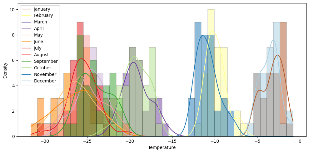
In this tutorial we define bias with respect to differences between the parameters that describe the PDFs of the time series. The PDF above is multi-modal, reflecting the seasonality of the data, meaning we’d need to use quite a few parameters to adequately describe the distribution. Simply using the mean would have limited value as we can see that the winter peak is ~5° higher for the climate model output while the summer peaks are approximately equal. The common approach here is to simply split the time series up by the month, focusing on defining bias for each month separately. The PDFs for individual months are approximately Gaussian (see below) and so the bias can be defined in terms of differences in the mean and variance parameters between the datasets.
In this tutorial, we’ll focus on just applying bias correction to the monthly June time series, shown below for the Manuela station.
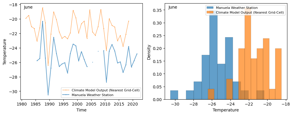
When examining the June time series, it’s clear that the climate model performs well at capturing the yearly variability and is highly correlated with the weather station output. However, there’s a significant bias in the mean of approximately 4°, indicating the utility of applying a bias correction.
Pairplots#
Since we’re interested in evaluating bias in the mean and variance of the June time series, it’s useful to think about predictors that have an influence on these metrics. The two most obvious predictors are elevation and latitude, both of which have well-understood physical justification for the impact on the mean temperature.
Filtering AWS Data:
We filter to just June records as discussed above and also to only stations with more than 5 records. This limits the influence of uncertainty in the empirical estimates used for exploratory analysis.
Nearest Grid Cells:
We’ve included a subcategory ‘Climate Model Nearest’ that represent values for just the climate model grid-cells nearest to each AWS. This is to get a feel for how representative the AWS samples are of Antarctic-wide region (e.g. it might be that differences between the datasets are just the result of the particular sample of locations with weather stations).
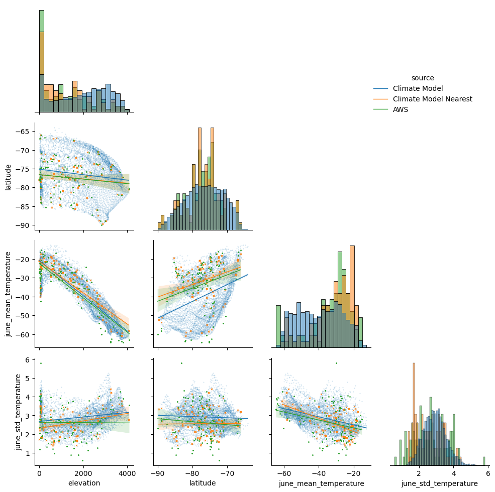
The pairplots bring up some interesting features:
Comparisons of the histograms between the ‘Climate Model’ data (all grid-cells over Antarctica) and the ‘Climate Model Nearest’ data (only grid-cells closest to the weather stations) indicate that the AWS sites are not a particularly representative sample of the whole Antarctic region. There’s a higher proportion of sites at zero elevation, clusters of sites at particular locations (and so latitudes), disproportionality high numbers of sites at regions with relatively high mean temperatures and relatively low standard deviations.
There are clear relationships between mean temperature with elevation and latitude. The slope of the linear relationship does not seem too strongly impacted by the particular subsample of AWS locations.
There’s only a weak relationship between the standard deviation in temperature with elevation and latitude. As a result we’ll leave out these predictors when estimating the standard deviation across the domain.
The behaviour of the relationship between elevation with mean temperature appears quite different at zero elevation sites, which could be linked with various factors such as the proximity and impact of the nearby sea on zero elevation sites. This potentially indicates at the utility of incorporating a distance to the coast predictor, although for this tutorial we leave this out.
Examining spatial covariance after removing influence of elevation and latitude#
The spatial pattern in mean temperature is currently dominated by the relationship with elevation and latitude. While these are clearly important predictors for mean temperature, it’s expected that there’ll be various other important factors that impact mean temperature but are harder to account for (e.g. the funnelling of wind down valleys will impact the mean temperature). One way of at least partially accounting for these factors is to model the spatial covariance between sites after removing the influence of elevation and latitude. That is that nearby sites are likely to be highly correlated as the factors impacting them are similar, whereas the further away you go the less correlated the sites will be (different valleys with different wind patterns etc).
Here we’ll plot the spatial pattern in the mean temperature after removing the linear influence of elevation and latitude. Additionally, we’ll plot the spatial pattern in the log of the standard deviation (taking the log to get the metric on the -\(\infty,\infty\) domain). Since the relationship between elevation and latitude with standard deviation appeared weak, we’ll ignore these predictors for this metric and simply remove a constant to get the zero-mean log(standard deviations).

It’s clear once we remove the linear dependency of temperature with elevation and latitude we get quite a different spatial structure for the mean temperature. This is the spatial structure we’ll want to model using Gaussian processes, where the covariance between nearby sites is captured by parameterising the covariance as a function of distance. In our model we’ll assume a single length scale for the covariance, that is to say we assume the covariance between nearby sites decays at the same distance wherever you are located over Antarctica. While this assumption is clearly broken in certain areas (e.g. covariance in steep regions near to the coast behaves differently to flat regions inland), it still provides a start and is a lot simpler than the approach of considering non-stationary lengthscales across the region (although this is possible). It’s important to consider how this will impact our results and we expect one of the main influences is that the noise term estimated for our Gaussian process will be relatively high to account for the sharp variations between nearby sites in particularly steep regions.
It’s also important to note that the spatial patterns in both the AWS data and climate model data are similar for each metric. That is the climate model is doing a reasonable job at capturing the more complex dependencies of mean temperature and log(standard dev) in temperature. To utilise this, in our model we consider a shared latent Gaussian process between the datasets and so predictions of the unbiased values are made conditioning on both datasets.
Examining spatial covariance in the bias#
It’s also useful to explore the spatial structure of the bias (both in the mean and log(standard deviation) of June temperature). In this exploratory analysis we do this by examining the empirical values of the metrics from the AWS data and the nearest climate model grid-cells.
For the mean temperature, this is done after accounting for the linear relationship with elevation and latitude (that is we examine the spatial structure in the bias of the residuals). For the log(standard deviation), we examine bias in the zero-meaned values for each dataset.
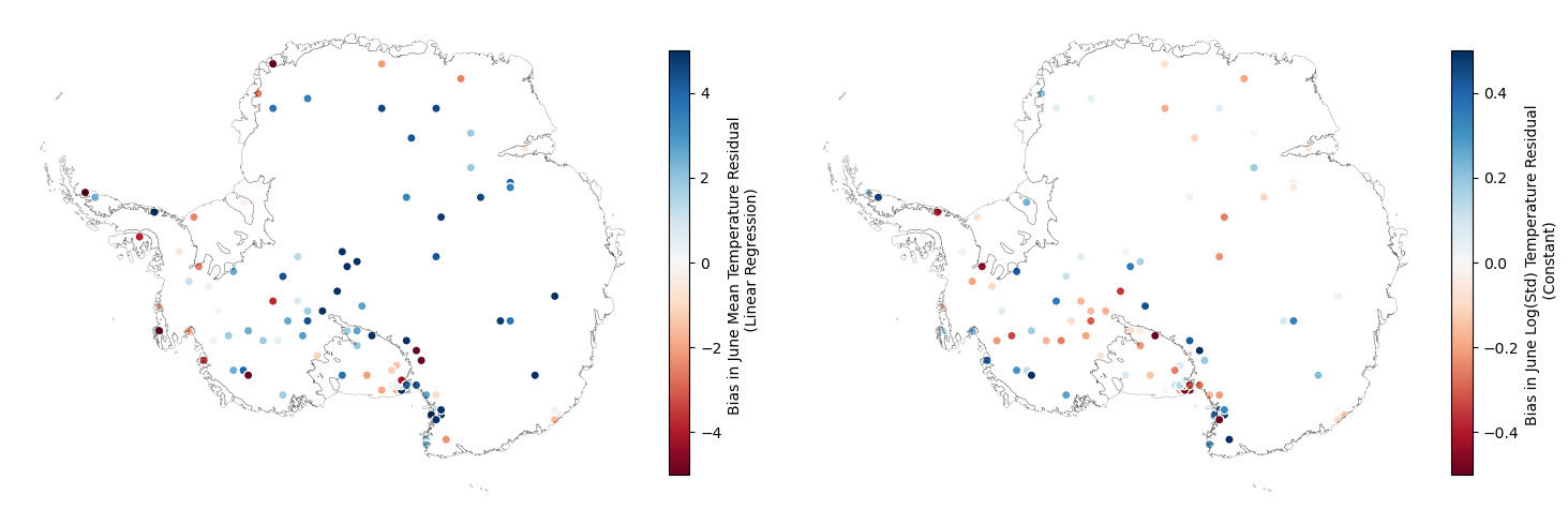
There’s clearly a spatial covariance pattern in the bias for both the mean and log(standard dev.). The length scale at which the covariance decays for the bias appears longer than for the raw value of the metrics of each dataset.
Examining relationships between variables and the bias in parameters#
It’s interesting to check whether there’s any obvious relationships between the biased parameter values and predictors such as elevation and latitude. Additionally, it’s worth checking if there’s a relationship between the biased and unbiased parameter values. We do this through a partial pairplot as shown below.
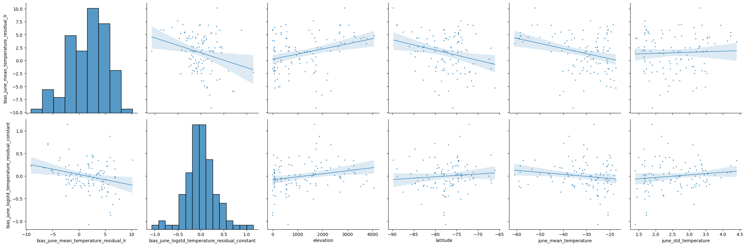
The above pairplot only shows weak relationships between the bias in parameters and the other variables. Therefore, in the model we’ll assume the bias is generated from an independent underlying process.
Data Preprocessing#
The main pre-processing steps we’ll do are simply scaling the elevation and latitude predictors and removing any AWS sites with only 2 records for average June temperature. We also define a random subsample of the climate model grid-cells, which we’ll use for inference on the parameters of the Gaussian processes in order to reduce the computational demands. Additionally, all the data is transformed away from Xarray and into a dictionary of device arrays (JAX versions of Numpy arrays) of the right shape that the inference package Numpyro expects.
Computational Complexity and Subsampling:
While Gaussian processes are extremely useful and flexible, their high computational demand of is often described as their Achilles’ heel. Typically, the time for inference scales as the cube of the number of data points, which is a result of taking the inverse of the covariance matrix when computing the likelihood of a set of data for given hyper-parameters. However, there are various methods for improving the speed of inference, such as sparse variational Gaussian processes (SVGPs). These are not utilised in this notebook as they require some additional complexity. Instead we do the sub-optimal procedure of simply only using a subsample of the climate model data for inference. This approach is clearly sub-optimal as it doesn’t target the regions of most interest, however, hopefully it’ll still produce sensible results and be sufficient for this tutorial example.
Additional Preprocessing:
Note that some pre-filtering has already been conducted to the data made available for the notebook, such as removing weather stations located on islands and filtering the climate model output to land onlu etc. These steps can be found in the preprocessing.py file of the notebook repository. Additionally, while not done in this notebook, it’s important to mention that typically feature engineering is an important component of preprocessing and we could for example derive a distance to the coast predictor.
It’s worth plotting the locations of the sampled climate model grid-cells and it’s also worth performing a quick sanity check that the data is in the right format:

Defining the model#
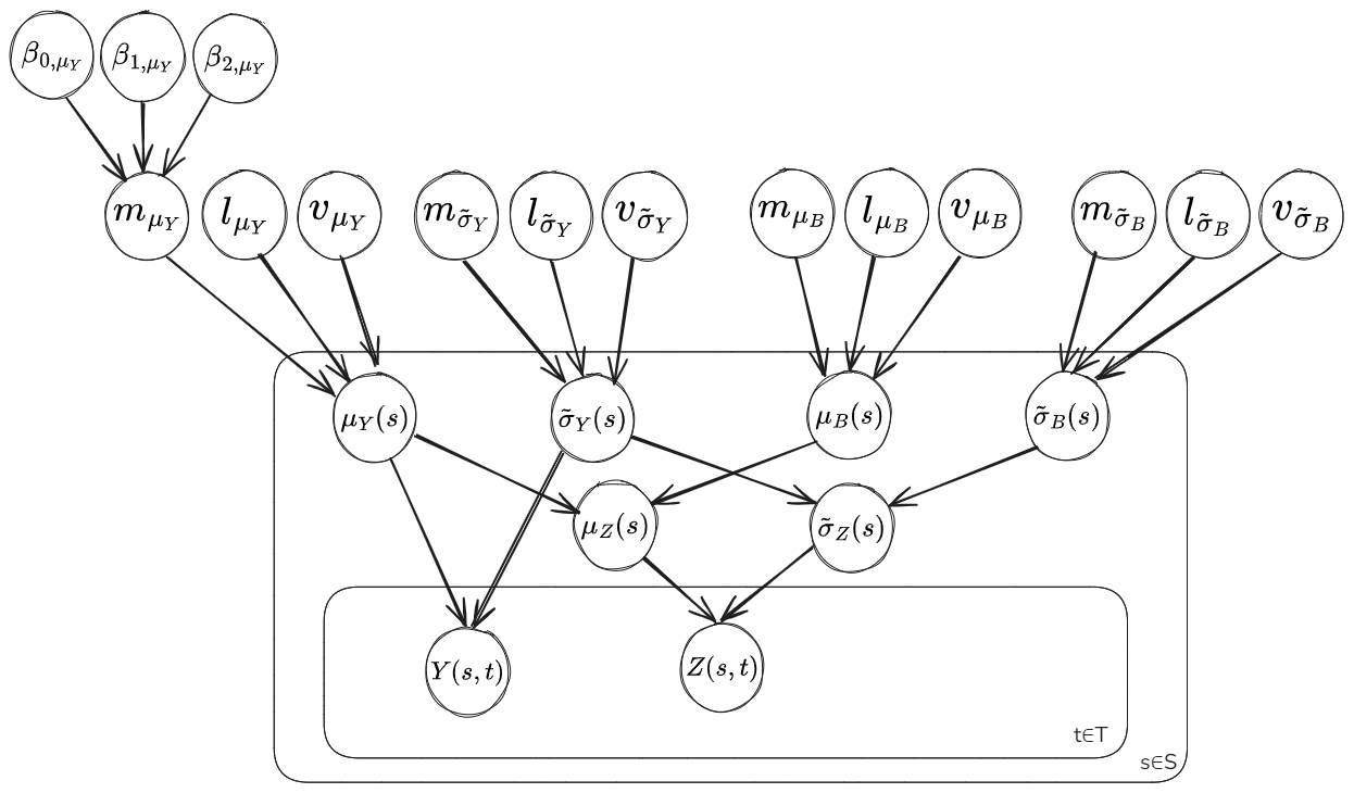
Let \(Y(s,t)\) represent the random variable for the June temperature from the AWS data at a particular time and location. Let \(Z(s,t)\) represent the equivalent but for the climate model output. We treat the marginal distribution of \(Y(s,t)\) and \(Z(s,t)\) as Normal, such that \(Y(s)\sim \mathcal{N}(\mu_Y(s),\sigma_Y(s))\) and \(Z(s)\sim \mathcal{N}(\mu_Z(s),\sigma_Z(s))\).
To model the spatial covariance in the parameters we use Gaussian processes. A log transformation is applied to the standard deviation (\(\tilde{\sigma}=log(\sigma)\)) so that it’s on the -\(\infty,\infty\) sample space of a Gaussian process. Shared latent Gaussian processes are considered between the datasets as well as an independent Gaussian process that generates the bias in the climate model output. The parameters for the climate model are then considered as the sum of an unbiased and biased component \(\mu_Z(s)=\mu_Y(s)+\mu_B(s)\) and \(\tilde{\sigma}_Z(s)=\tilde{\sigma}_Y(s)+\tilde{\sigma}_B(s)\), where each component is modelled as generated from a Gaussian process. The Gaussian processes are parameterised by a mean function and covariance function. The mean function for \(\mu_Y(s)\) is considered linear with respect to elevation and latitude, while for the other parameters it is considered a constant. The covariance function is taken as a Matern3/2 kernel with a lengthscale \(l\) and variance \(v\).
The plate diagram below shows the relational dependence between the parameters of the model.
Mean Function and Covariance Function:
The mean function for the parameter \(\mu_Y(s)\) is taken as \(m_{\mu_Y}(s)=\beta_{0,\mu_Y} + \beta_{1,\mu_Y} \cdot x_{ele}(s) + \beta_{2,\mu_Y} \cdot x_{lat}(s)\).
The covariance function is taken as a Matern3/2 kernel for each parameter, that is: \(k_{M^{3/2}}(s,s')=v\left(1+\dfrac{\sqrt{3}|s-s'|}{l}exp\left({-\dfrac{\sqrt{3}|s-s'|}{l}}\right)\right)\). The distance \(|s-s'|\) between points is computed from the ‘grid_latitude’ and ‘grid_longitude’ coordinates, which are approximately Euclidean across the domain. The matern3/2 kernel is a popular choice for real-world data applications, see this blog by Andy Jones for some additional info: The Matérn class of covariance functions .
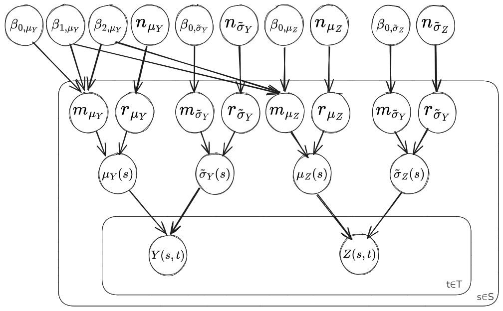
Splitting up the model for computation#
It’s quite common when using Gaussian processes to fit the mean function independently of the covariance function. That is to say a mean function is fit to the data initially and then the zero-mean data is fit using the GP implementation that handles covariances between points. There are various reasons for this, such as making the covariance matrix more well-conditioned for inference.
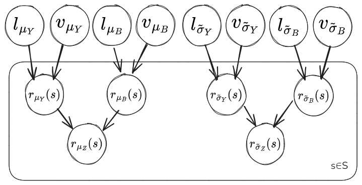
In this notebook we’ll split up the model into a first component estimating the parameters \(\mu_Y(s_Y)\), \(\mu_Z(s_Z)\), \(\tilde{\sigma}_Y(s_Y)\) and \(\tilde{\sigma}_Z(s_Z)\) at the AWS and climate model grid cell locations, along with the global parameter values for the mean functions of the latent Gaussian processes \(\beta_{0,\mu_Y}\), \(\beta_{1,\mu_Y}\), \(\beta_{2,\mu_Y}\), \(m_{\mu_B}\), \(m_{\tilde{\sigma}_Y}\) and \(m_{\tilde{\sigma}_B}\). Then the second component will use the residuals \(r_{\mu_Y}(s_Y)\), \(r_{\mu_Z}(s_Z)\), \(r_{\tilde{\sigma}_Y}(s_Y)\) and \(r_{\tilde{\sigma}_Z}(s_Z)\) to estimate the parameters of the covariance function for the latent Gaussian processes \(l_{\mu_Y}\), \(v_{\mu_Y}\), \(l_{\mu_B}\), \(v_{\mu_B}\), \(l_{\tilde{\sigma}_Y}\), \(v_{\tilde{\sigma}_Y}\), \(l_{\tilde{\sigma}_B}\) and \(v_{\tilde{\sigma}_B}\).
Modelling assumptions and splitting up the model:
It’s important to consider the impact of splitting up the hierarchical model and what assumptions it makes. The main assumption we make is that the noise in \(\mu_Y(s_Y)\), \(\mu_Z(s_Z)\), \(\tilde{\sigma}_Y(s_Y)\) and \(\tilde{\sigma}_Z(s_Z)\) is Gaussian, which seems reasonable. However, if we expected the posterior distributions of these parameters to be highly skewed and non-Gaussian then splitting up the model wouldn’t adequately capture this and keeping a hierarchical model would better represent the uncertainty in the final predictive distributions.
Model Diagram Component 1: Mean Function:
Model Diagram Component 2: Residuals and Covariance
Parameter Inference#
Inference is performed on the two components of the model separately. To limit the runtime of this notebook, we’ll provide the code for running the inference but will perform the actual inference separately and load in the output to examine. The python scripts for running the inference separately and saving the output are available via the jupterbook_render branch of the repository. Loading in the inference data:
url = ("https://zenodo.org/records/14779669/files/data_dictionary.pkl?download=1")
filename = f'{data_path}data_dictionary.pkl'
if os.path.exists(filename):
    print('File already exists')
else:
    urlretrieve(url, filename)
    print('File downloaded')
File already exists
Inference on parameters of the mean function#
Utilising the Numpyro python package to define the model for component 1:
In the model definition ‘omean’ represents the mean June temperature estimate at each AWS location, while ‘cmean’ is the the equivalent for the climate model output at the grid-cell locations. Similarly, ‘ologvar’ and ‘clogvar’ represents for the log-variance for each dataset and location respectively. The model follows the following equations:
Defining a function for running the Bayesian inference on the model parameters given the data:
As we’re utilising a Bayesian framework, we’ll have to define some prior distributions for the parameters. While in theory the prior distribution should represent our state of knowledge before observing the data and so if we have no additional knowledge should be fully non-informative, in practice it’s common to at least set sensible bounds using the exploratory analysis to limit the complexity of the inference space. Here, we compute some basic metrics, which we then use to help set sensible priors.
The code for running the inference and saving estimates of the parameter posterior distributions is given below. Note that the code is commented out as instead of running the inference within this notebook, for computational reasons we’ll simply load in the output. The output is saved using the ArViZ package, which handles inference data from lots of different probabilistic programming packages and can be used to produce nice summary metrics and plots.
MCMC is an approximate procedure and it is difficult to assess directly whether the samples returned from the inference accurately capture the true posterior distributions of the parameters. The effective sample size (ESS) and r_hat diagnostics provide some indication, we’re looking for values of r_hat in the range (1.0, 1.05) and ESS that are comparable to the total number of samples, which we get in this run:
| mean | sd | hdi_2.5% | hdi_97.5% | mcse_mean | mcse_sd | ess_bulk | ess_tail | r_hat | |
|---|---|---|---|---|---|---|---|---|---|
| omean_b0 | -33.416 | 0.539 | -34.523 | -32.402 | 0.005 | 0.007 | 13604.0 | 5746.0 | 1.0 |
| omean_b1 | -10.059 | 0.069 | -10.193 | -9.926 | 0.001 | 0.001 | 11527.0 | 6119.0 | 1.0 |
| omean_b2 | 3.100 | 0.068 | 2.963 | 3.234 | 0.001 | 0.001 | 16561.0 | 6066.0 | 1.0 |
| omean_noise | 6.740 | 0.402 | 5.978 | 7.514 | 0.004 | 0.006 | 12338.0 | 5185.0 | 1.0 |
| ologvar_b0 | 2.043 | 0.066 | 1.917 | 2.174 | 0.001 | 0.001 | 6133.0 | 6362.0 | 1.0 |
| ologvar_noise | 0.584 | 0.063 | 0.467 | 0.710 | 0.001 | 0.001 | 2558.0 | 4297.0 | 1.0 |
| cmean_b0 | -32.623 | 0.084 | -32.796 | -32.464 | 0.001 | 0.001 | 11574.0 | 5437.0 | 1.0 |
| cmean_noise | 5.263 | 0.050 | 5.164 | 5.361 | 0.000 | 0.001 | 16003.0 | 5160.0 | 1.0 |
| clogvar_b0 | 2.146 | 0.006 | 2.135 | 2.158 | 0.000 | 0.000 | 9323.0 | 6671.0 | 1.0 |
Inference on parameters of the residual and covariance functions#
For component 2 of the model, the residuals of the mean and log(standard dev.) are treated as independent and so inference can be conducted separately for each. Again utilising the Numpyro python package to define the model gives:
In the model definition for the residuals the observations are the expectations of the residuals computed from inference of the meanfunction model in component 1. That is \(E[r_{\mu_Y}(s_Y)]\) and \(E[r_{\mu_Z}(s_Z)]\). The uncertainty in these values is captured through the variance, so \(V[r_{\mu_Y}(s_Y)]\) and \(V[r_{\mu_Z}(s_Z)]\). Although, we don’t include \(V[r_{\mu_Z}(s_Z)]\) in the model definition as it’s an insignificant quantity. The model follows the equations:
Function ‘generate_obs_conditional_climate_dist’:
The function ‘generate_obs_conditional_climate_dist’ is defined as the parameters of \(\mathcal{GP}(0|,k(s,s'|l_{\mu_Y},v_{\mu_Y},n_{\mu_Y}))\) and \(\mathcal{GP}(0|,k(s,s'|l_{\mu_B},v_{\mu_B},n_{\mu_B}))\) are conditional on both \(r_{\mu_Y}(s_Y)\) and \(r_{\mu_Z}(s_Z)\). So we generate a distribution for the probability of the unbiased AWS data given the already conditioned on climate model data.
Again choosing sensible priors for the parameters of the model that have reasonable bounds based on some basic summary metrics:
The code for running the inference and saving estimates of the parameter posterior distributions is given below. Note that the code is commented out as instead of running the inference within this notebook, for computational reasons we’ll simply load in the output.
Parameter Inference for Model of Mean Residuals
| mean | sd | hdi_2.5% | hdi_97.5% | mcse_mean | mcse_sd | ess_bulk | ess_tail | r_hat | |
|---|---|---|---|---|---|---|---|---|---|
| bkern_var | 5.838 | 7.004 | 0.102 | 18.185 | 0.125 | 0.311 | 2838.0 | 1879.0 | 1.0 |
| blengthscale | 12.991 | 4.687 | 4.797 | 19.994 | 0.075 | 0.053 | 3111.0 | 1959.0 | 1.0 |
| bnoise | 0.604 | 0.510 | 0.101 | 1.622 | 0.008 | 0.013 | 2689.0 | 1391.0 | 1.0 |
| kern_var | 35.067 | 9.148 | 20.810 | 53.265 | 0.263 | 0.537 | 2067.0 | 1227.0 | 1.0 |
| lengthscale | 3.431 | 0.638 | 2.308 | 4.641 | 0.016 | 0.019 | 2015.0 | 1571.0 | 1.0 |
| noise | 5.468 | 1.086 | 3.384 | 7.638 | 0.020 | 0.018 | 3129.0 | 2633.0 | 1.0 |
Parameter Inference for Model of LogVar Residuals
| mean | sd | hdi_2.5% | hdi_97.5% | mcse_mean | mcse_sd | ess_bulk | ess_tail | r_hat | |
|---|---|---|---|---|---|---|---|---|---|
| bkern_var | 0.067 | 0.064 | 0.010 | 0.184 | 0.001 | 0.003 | 2827.0 | 1632.0 | 1.0 |
| blengthscale | 13.684 | 4.219 | 6.214 | 19.997 | 0.076 | 0.048 | 2552.0 | 1915.0 | 1.0 |
| bnoise | 0.013 | 0.003 | 0.010 | 0.019 | 0.000 | 0.000 | 2291.0 | 1534.0 | 1.0 |
| kern_var | 0.125 | 0.075 | 0.044 | 0.250 | 0.002 | 0.006 | 1939.0 | 1116.0 | 1.0 |
| lengthscale | 5.598 | 1.638 | 3.142 | 8.781 | 0.045 | 0.075 | 1974.0 | 1236.0 | 1.0 |
| noise | 0.012 | 0.002 | 0.010 | 0.017 | 0.000 | 0.000 | 3033.0 | 1774.0 | 1.0 |
The posterior distributions for the parameters of the model appear sensible on first glance. The r-hat statistic indicates that the chains are independent as desired and the effective sample size is of comparable magnitude to the total number of samples taken.
Making posterior predictive estimates of the unbiased mean and variance across the domain#
From the previous section we have:
Posterior estimates of the mean and log-variance at the AWS sites and climate model grid cells, that is \(\mu_Y(s_Y)\), \(\tilde{\sigma}_Y(s_Y)\), \(\mu_Z(s_Z)\) and \(\tilde{\sigma}_Z(s_Z)\). As well as the estimates for the meanfunction and residual components: \(m_{\mu_Y}(s_Y)\), \(m_{\tilde{\sigma}_Y}(s_Y)\), \(m_{\mu_Z}(s_Z)\), \(m_{\tilde{\sigma}_Z}(s_Z)\) and \(r_{\mu_Y}(s_Y)\), \(r_{\tilde{\sigma}_Y}(s_Y)\), \(r_{\mu_Z}(s_Z)\) and \(r_{\tilde{\sigma}_Z}(s_Z)\).
Posterior estimates of the parameters of the mean functions, so \(\beta_{0,\mu_Y}\), \(\beta_{1,\mu}\), \(\beta_{2,\mu}\), \(\beta_{0,\mu_Z}\), \(\beta_{0,\tilde{\sigma}_Y}\) and \(\beta_{0,\tilde{\sigma}_Z}\).
Posterior estimates of the parameters of the covariance functions, so \(l_{\mu_Y}\), \(v_{\mu_Y}\), \(n_{\mu_Y}\), \(l_{\mu_B}\), \(v_{\mu_B}\) and \(n_{\mu_B}\).
Now we want to make estimates of the posterior distributions of the unbiased mean and log-variance at the climate model locations to use for bias correction, so \(\mu_Y(s_Z)\) and \(\tilde{\sigma}_Y(s_Z)\). This is known as the posterior predictive and involves conditioning on both the inferred parameters of the model and the observed data. Since we split up the hierarchical model, to get \(\mu_Y(s_Z)\) and \(\tilde{\sigma}_Y(s_Z)\) we’ll get estimates for \(m_{\mu_Y}(s_Z)\) and \(m_{\tilde{\sigma}_Y}(s_Z)\) from the first component of the model, then \(r_{\mu_Y}(s_Z)\) and \(r_{\tilde{\sigma}_Y}(s_Z)\) from the second component.
Posterior predictive calculation:
Let the collection of parameters for the model be: \(\phi = [m_{\mu_Y}(s_Y), m_{\mu_Z}(s_Z), r_{\mu_Y}(s_Y), r_{\mu_Z}(s_Z), \beta_{0,\mu_Y}, \beta_{1,\mu}, \beta_{2,\mu}, \beta_{0,\mu_Z}, l_{\mu_Y}, v_{\mu_Y}, n_{\mu_Y}, l_{\mu_B}, v_{\mu_B}, n_{\mu_B}]\)
Then the posterior predictive distributions is given by:
Where \(p(m_{\mu_Y}(\hat{s})|\beta_{0,\mu_Y}, \beta_{1,\mu}, \beta_{2,\mu}, \beta_{0,\mu_Z})\) is the predictive distribution of the meanfunction and \(p(r_{\mu_Y}(\hat{s})|r_{\mu_Y}(s_Y), r_{\mu_Z}(s_Z),l_{\mu_Y}, v_{\mu_Y}, n_{\mu_Y}, l_{\mu_B}, v_{\mu_B}, n_{\mu_B})\) is the predictive distribution of the residual function. The distribution \(p(\theta|Y(s_Y),Z(s_Z))\) is simply the posterior distribution for the parameters of our model, which we get samples from using MCMC.
To get samples of \(\mu_Y(\hat{s})\) from the posterior predictive distribution we take samples from the predictive distribution of the meanfunction and the predictive distribution of the residual using parameters sampled from the posterior. That is for each sample from our MCMC inference, we define the predictive distributions and then take a sample.
Sampling the predictive distribution of the mean function is simple:
Sampling the predictive distribution of the residual is more difficult and we construct some functions to help.
Generating the residual posterior predictive samples:
Computing the expectations and uncertainties:
Results#
To plot the predictions of the unbiased mean and log(variance), as well as the bias, we combine the posterior predictives with a dataset containing the relevant coordinates for plotting:
The expectation of the unbiased and biased June mean temperature at the climate model grid-cell locations is then given below along with the uncertainty. The values are the result of summing the posterior predictive estimates from both components of the model.
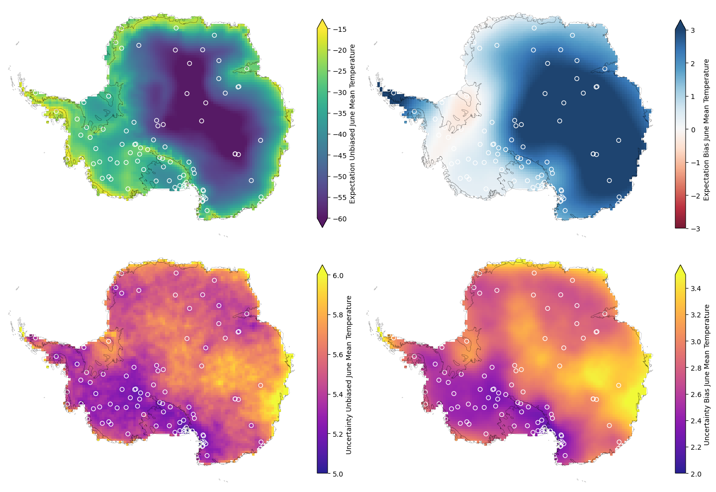
The equivalent for the log(variance) is also given below:

There are various interesting things to note about these predictions:
The expectation for the bias varies smoothly across the domain, which is the result of modelling it with a single lengthscale in the latent Gaussian process. In reality we know the bias will vary more sharply across the region, however with limited data capturing the large scale patterns is already a good start and the smoothness makes it clear we’re not overfitting to the data. Being resistant to overfitting is a common benefit of Gaussian processes.
The uncertainty is dominated by a constant noise term across the domain, which makes sense since we expect sharp variations that are difficult to predict with the limited weather station data available.
The uncertainty is lowest nearby clusters of weather stations. This makes sense and is the result of modelling the spatial covariance. Away from weather stations we have limited information about the bias.
Quantile Mapping#
The final step after estimating the unbiased PDF parameter values across the domain is to actually apply the bias correction to the original climate model spatio-temporal output. To do this we utilise quantile mapping, which maps the climate model data onto the CDF represented by the unbiased PDF parameters.
For every record \(j\) at each location \(i\) we apply the mapping: $\(\hat{z}_{s_{i,j}} = F_{Y_{s_i}}^{-1}(F_{Z_{s_i}}(z_{s_{i,j}}))\)$
Where \(F_{Y_{s_i}}^{-1}\) is the unbiased inverse cumulative density function and \(F_{Z_{s_i}}\) is the CDF for the climate model data.
Instead of using the expectation of posterior predictive parameter estimates, realisations of the posterior predictives of the unbiased parameters are utilised and quantile mapping performed with each realisation separately. This allows propagation of uncertainty, producing multiple realisations for the corrected timeseries and thus an uncertainty band on the correction. To illustrate this six AWS sites are chosen and the timeseries from the AWS records plot alongside the timeseries for the original and corrected climate model output from the nearest grid cell. Additionally, the original and bias corrected climate model timeseries are shown for a site isolated from any nearby AWSs.
Taking a selection of 6 weather station sites dotted around the domain and 1 isolated site, we’ll demonstrate the bias corrected time series at each of the nearest climate model grid-cells. To start with we’ll show the locations of the different chosen sites. Then we’ll illustrate the time series for the weather stations at the sites, the time series for the climate model output of the nearest grid-cell and the time series of the bias corrected climate model output for the nearest grid-cell.
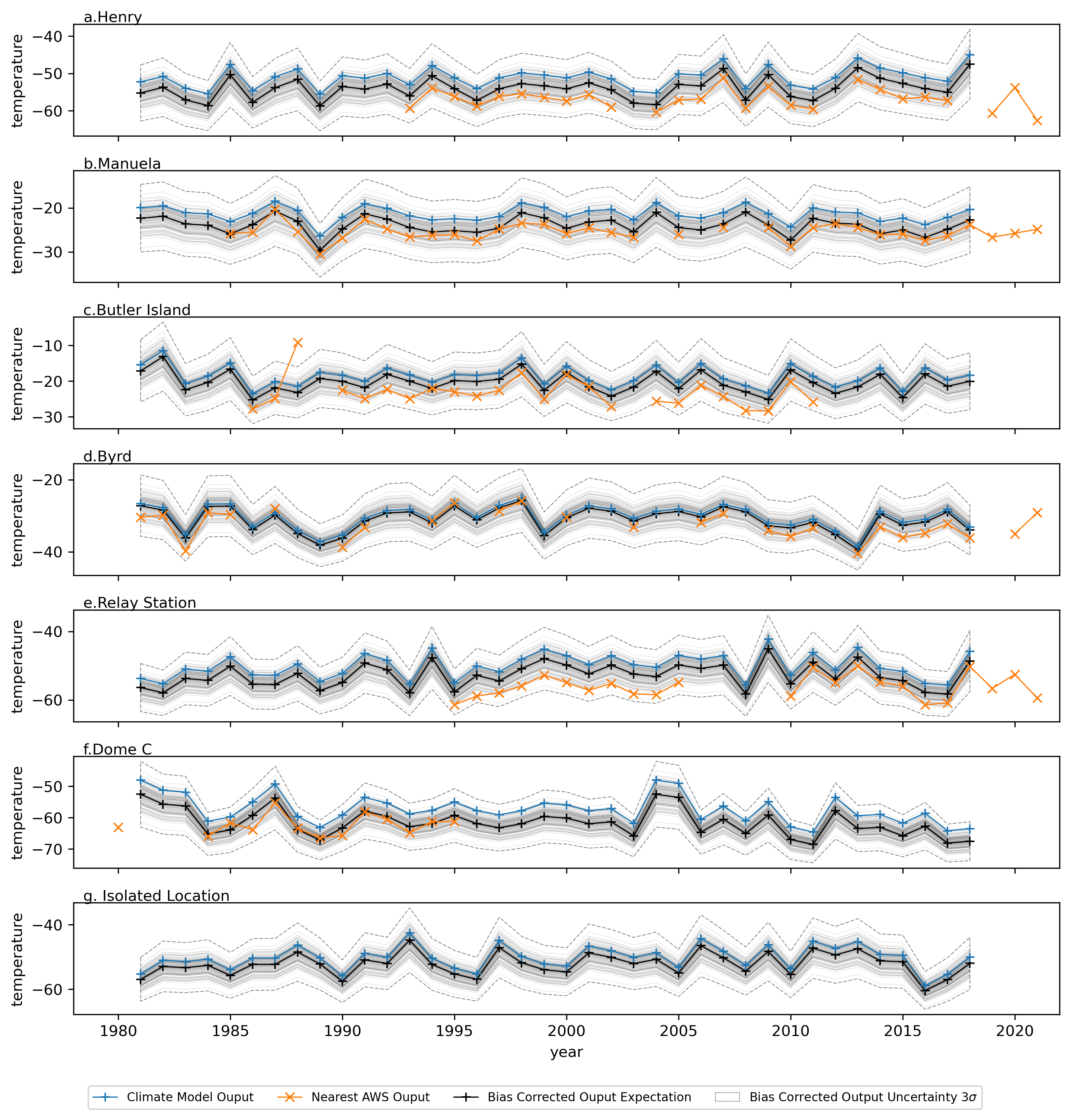
The bias correction seems to be performing reasonably, with a general shift of the time series towards that of the nearby unbiased weather station data and realistic uncertainty bands. It’s also worth noting some interesting features visible in the weather station data including:
An apparent temperature anomaly in the Butler Island records;
An apparent shift in the mean after a break for the Relay station.
It is likely these are instrumentation errors rather than physically meaningful phenomenon that need to be captured. This would be best resolved with further data preprocessing and highlights the importance of understanding specific features of the real-world data that are hard to account for in modelling. In general the assumption of time-invariant bias seems reasonable and the model is adding value by improving the timeseries agreement with the observed values and by introducing an uncertainty that can be propagated further through physical ice models, providing some range of possible outcomes, which in turn might be used in various cost-decision analysis schemes.
Conclusions#
Hopefully this notebook provides some interesting ideas that are generalisable to many areas of application including:
Where we care about uncertainty in the end output and creating a flexible modelling framework that propagates uncertainty in the different components and is explicit about the assumptions made through prior distributions.
Where we’re trying to combine multiple datasets with different spatial and temporal coverage.
Where we want to explicitly model the underlying covariance between points.
The main limitations of the methodology presented are in the computational complexity of inference. The model in its current form runs slowly even for small datasets such as presented in this notebook. This makes iterative improvements and careful testing of the results challenging. There are various options to speed up the code that still need exploring and if you’re interested in contributing please do so through the repository link. Another important limitation of the code as it stands is that it’s currently lacking rigorous unit testing of functions and that the documentation needs improving. As such it is suggested to takeaway components of the pipeline to utilise on your own projects and to supplement that with official examples from the relevant package repositories such as Numpyro and TinyGP.