{targets}: a data pipeline tool for R

class: center, middle, inverse, title-slide

.title[
# {targets}: a data pipeline tool for R
]
.author[
### Peter Levy, UKCEH Edinburgh
]

---

---
background-image: url("./images/unstructured.png")
background-position: 90% 50%
background-size: 300pt

## A typical unstructured manual workflow

- get some data
--

- write some code
--

- produce graphs & tables
--

- paste into Word document
--

- write some text
--

- 
--

- *come back a month later*
--

- *forget what you actually did*
--

- *re-run? re-do from scratch?*
--

**No declared structure**

**Dependencies not obvious**

---

## A Workflow: interconnected tasks

???

A large workflow has a large number of moving parts. We have datasets that we preprocess or simulate, analyses of those datasets, and summaries of the analyses.

---

## Changes

???

If you change any one of these parts - whether it is a bugfix, a tweak to a model, or some new data -

---

## Consequences?

???

Then everything that depends on it is no longer valid, and you need to rerun the computation to bring the results back up to date. This is seriously frustrating when you're in development and you're still making a constant stream of changes to code and data in real time. If every change means you need to rerun the project, there is no way the results can keep up...

---

## Changes

---

## Consequences?

---

## Changes

---

## Consequences?

---

## A more structured workflow ...

```
run_everything.R
R/
├── 01-read_data.R
├── 02-wrangle.R
├── 03-model.R
├── 04-results.R
└── 05-plot.R
└── 06-paper.Rmd
data/
└── input_data.csv
```

### Problems

- computation may take hours or days
- has anything changed since last run?
- no guarantees
- what ramifications?

???

Move away from numbered scripts and R Markdown as a way to manage the computation end to end. It is an okay strategy for small projects, but it falls apart quickly as a project grows.

---

background-image: ./images/not.png

## <img src="./images/no.png" width="40" height="40"> A more structured workflow ...

```
run_everything.R
R/
├── 01-read_data.R
├── 02-wrangle.R
├── 03-model.R
├── 04-results.R
└── 05-plot.R
└── 06-paper.Rmd
data/
└── input_data.csv
```

### Problems

- computation may take hours or days
- has anything changed since last run?
- no guarantees
- what ramifications?

---

## Dilemma: short runtimes or reproducible results?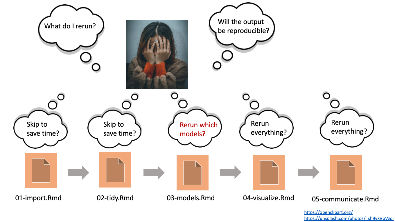

![](./images/decisions.png)

---

class: middle, bottom
background-image: url(./images/logo.png)
background-size: contain

---

## {targets}: formally declare structure of workflow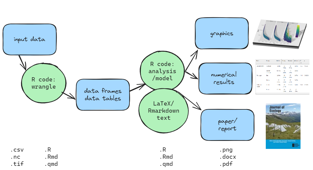

![](./images/pipeline1.png)

---

## {targets}: formally declare structure of workflow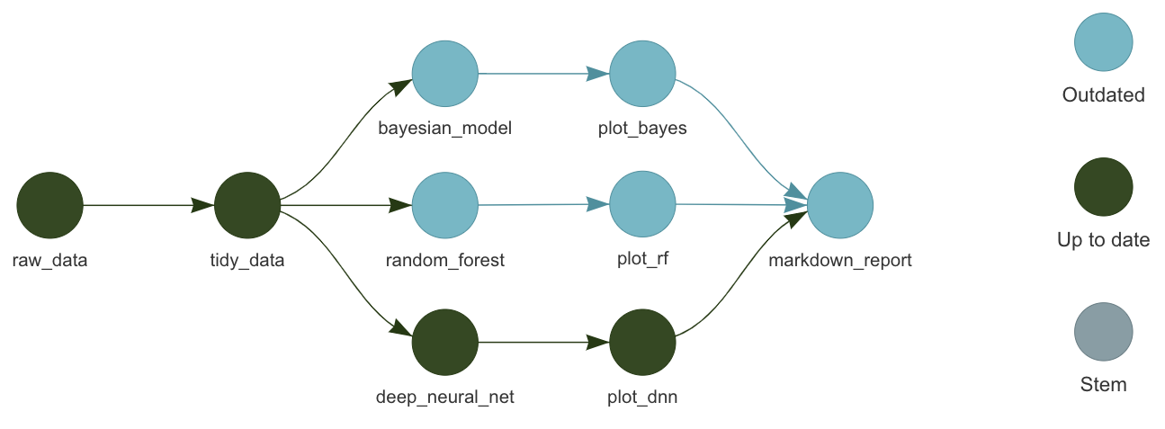

![](./images/pipeline_graph.png)

- Define pipeline:
    - R objects (*targets*) modified by functions
- Automatic analysis of dependencies
    - functions, data, files
- Figures out what to re-run.
    - Only runs out-of-date targets
- Ensures computational reproducibility.

---

## {targets}

* Supports (enforces) a function-oriented programming style
* Automatically manages data

* Fundamentally designed for R
* Options available for python:
    - `snakemake`
    - ...

---

## Typical minimal project structure

```r
*_targets.R # Required top-level configuration file
R/
└── functions.R
data/
└── data.csv
```

- Not restrictive, many variations on this theme

???

You can organize your functions however you want, but it's common practice to put them in scripts inside an R/ folder. Similarly, input datasets can go anywhere, but a data/ folder just helps keep things clean.

And at this point, you have a good clean function-oriented project. Even if you decide not to use targets, this function-oriented style still has a lot of value. However, if you're thinking about using targets, then converting to functions is almost all of the work. Once you've done that, you're already almost there. All you need now is to outline the specific steps of the computation in a formal pipeline. And that's where this _targets.R script comes into play. It always lives at the root of the project, and it's always called "_targets.R".

---

## Typical minimal project structure

```r
_targets.R # Required top-level configuration file
R/
*└── functions.R
data/
└── data.csv
```

- Not restrictive, many variations on this theme
- Can include both code and text in markdown/LaTeX

---

## Define pipeline as a list of targets

```r
# _targets.R
library(targets)
tar_option_set(packages = c("readr", "dplyr", "ggplot2"))
# Run the R scripts in the R/ folder with your custom functions:
tar_source()
list(
  tar_target(filename, "data.csv", format = "file"),
  tar_target(data, get_data(filename)),
  tar_target(model, fit_model(data)),
  tar_target(plot, plot_model(model, data))
)
```

???

The purpose of _targets.R is to set up the project at a high level. It loads the packages required to define the pipeline, it loads your custom functions and global objects, it sets high-level options such as the packages the targets are going to need, and it defines the pipeline at the very end.

At the bottom of _targets.R, you list out objects called targets. Each target is an individual step in the workflow. It has an informative name like "sim" or "patients", and it has a R command that invokes your custom functions and returns a value.

---

## targets understands code and data dependencies.

```r
tar_visnetwork()
```
<center>
<img src="images/graph5.png", height = "350px" align="middle" style="border: none; box-shadow: none; text-align: center;">
</center>

???

It's always good practice to visualize the dependency graph of the plan. targets has functions to do this for you, and it really demystifies how the package works. So here you see the flow of the project from left to right. We reproducibly track an input data file, we load that data to split into training and test, and we prepare that data for the models using a Tidymodels recipe.

But how does targets deduce this flow? How does it know that the churn_recipe depend on churn_data? The order you write targets in the pipeline does not matter. targets knows that churn_recipe depends on churn_data because the symbol "churn_data" is mentioned in the command for "churn_recipe" in the pipeline. targets scans your commands and functions without actually running them it in order to look for changes and understand dependency relationships. This is called static code analysis.

---

## Build your targets.

```r
tar_make()
```

```
#> ▶ dispatched target filename
#> ● completed target filename [0 seconds]
#> ▶ dispatched target data
#> New names:
#> ● completed target data [0.06 seconds]
#> ▶ dispatched target model ● completed target model [0 seconds]
#> ▶ dispatched target plot
#> ● completed target plot [0.02 seconds]
#> ▶ ended pipeline [0.42 seconds]
#> • `` -> `...1`
```

???

To actually run the workflow, we use a function called tar_make(). tar_make() creates a clean new reproducible R process, runs _targets.R to populate the new session and define the pipeline, resolves the dependency graph, runs the correct targets in the correct order from the dependency graph, and writes the return values to storage.

---

## Check the targets produced

- `tar_load()` and `tar_read()` get targets from the `_targets/` data store.

```r
tar_read(plot)
```

???

Afterwards, all the targets are in storage. There's a special key-value store in a hidden _targets/ folder, and targets has functions tar_load() and tar_read() to retrieve data from the store. targets abstracts artifacts as ordinary objects. You don't need to worry about where these files are located, you just need to know the target names. This is the exploratory analysis phase. Always inspect your targets for issues between calls to tar_make().

---

## Previous work is still up to date.

```r
tar_outdated()
```

```
#> character(0)
```

```r
tar_make()
```

```
#> ✔ skipped target filename
#> ✔ skipped target data
#> ✔ skipped target model
#> ✔ skipped target plot
#> ✔ skipped pipeline [0.15 seconds]
```

???

So when we run the pipeline again, only the models run. The tool skips the data targets because they are already up to date.

---

## Resources

* Get [`targets`](https://github.com/ropensci/targets):

```r
install.packages("remotes")
remotes::install_github("ropensci/targets")
```

* Tutorial materials: <https://github.com/wlandau/targets-tutorial>
* Development repository: <https://github.com/ropensci/targets>
* Full user manual: <https://books.ropensci.org/targets/>
* Reference website: <https://docs.ropensci.org/targets/>

* These slides: <https://github.com/NERC-CEH/targets_demo>

???

There are several resources to learn about targets. There's a reference website, an online user manual, and a repository with the example code from today.

targets is nearing the end of its beta phase. I am about to submit it to rOpenSci for peer review, and I hope to have it on CRAN at the end of this year or early next year. Now is a great time for feedback because there is no formal release yet and the interface is not yet set in stone.

---

## Advanced topics

- Parallelisation
- Use with Rmarkdown

- 'Projects' - inter-linked pipelines
- Branching - targets generated dynamically at run time

---

## Parallelisation

- {targets} understands inter-dependence
- works out which can be run in parallel
- several options
     - `future` package is easiest

```r
library(future)
future::plan("multicore")
```

Run targets objects in parallel with 3 processors:

```r
tar_make_future(workers = 3L)
```

---

## Use with Rmarkdown

Include rendering of markdown in pipeline with:

```r
tar_render(target_name, filename.Rmd)
```

Include target objects in markdown document with:

```r
tar_read(target_name)
```

---

## A real example

```r
library(targets)
library(tarchetypes)
library(here) # construct file paths relative to project root
library(fs) # file system operations

library(future) # for parallelisation
future::plan("multicore")
v_pkgs <- c("qs", "tidyverse", "readxl", "data.table", "spCEH", "units",
    "rayshader", "viridis", "scales", "sf", "gridExtra", "MuMIn",
    "ggforce", "ggeffects", "lme4", "brms", "ConsReg")
    
tar_option_set(
  packages = v_pkgs,
  format = "qs"
)

# Functions used by the targets.
source(here::here("R", "dsdz.R"))
...
)
```

---

## A real example

```r
# List of targets
list(
  # data files:
  tar_target(fname_eb_2015, here("data-raw/EasterBush/EB_soil_long_2015_09_23.csv"), format = "file"),
  tar_target(fname_eb_2012, here("data-raw/EasterBush/EB_soil_core_CN_2012.csv"), format = "file"),
  tar_target(fname_elum,    here("data-raw/ELUM", "ELUM soil carbon data.xlsx"), format = "file"),
  tar_target(fname_rac ,    here("data-raw/RAC", "HS2 soil carbon data_additional samples_JUly 2022.xlsx"), format = "file"),
  tar_target(fname_ward ,   here("data-raw/Ward", "1. FINAL All data at 5 depth increments - Copy.xls"), format = "file"),
  tar_target(fname_ward_coord, here("data-raw/Ward", "SITE DETAILS 2008.xls"), format = "file"),
  tar_target(fname_brad, here("data-raw/Bradley", "UK_Soil_Series_2005.csv"), format = "file"),
  tar_target(fname_brad_summary, here("data-raw/Bradley/Bradley_2005_summary.csv"), format = "file"),
  tar_target(fname_cs_1978, here("data-raw/CS", "CS1978_SOIL_PHYSICOCHEM.csv"), format = "file"),
  tar_target(fname_cs_1998, here("data-raw/CS", "CS1998_SOIL_PHYSICOCHEM.csv"), format = "file"),
  tar_target(fname_cs_2007, here("data-raw/CS", "CS2007_SOIL_PHYSICOCHEM.csv"), format = "file"),
  tar_target(fname_cs_2019, here("data-raw/CS", "CS2019_20_21_Pete.xlsx"), format = "file"),
  tar_target(fname_gmep, here("data-raw/GMEP", "GMEP_SOIL_METRICS_2013_16.csv"), format = "file"),
  
  # wrangle data files:
  tar_target(dt_eb  , wrangle_eb(  fname_eb_2015, fname_eb_2012)),
  tar_target(dt_elum, wrangle_elum(fname_elum)),
  tar_target(dt_rac , wrangle_rac(fname_rac)),
  tar_target(dt_ward, wrangle_ward(fname_ward, fname_ward_coord)),
  tar_target(dt_brad, wrangle_brad(fname_brad)),
  tar_target(dt_cs ,  wrangle_cs(fname_cs_1978, fname_cs_1998, fname_cs_2007)),
```

---

## A real example

```r
  tar_target(dt_cs2019, wrangle_cs2019(fname_cs_2019)),
  tar_target(dt_gmep, wrangle_gmep(fname_gmep)),
  tar_target(dt_all , rbind(dt_eb, dt_elum, dt_rac, dt_ward, dt_brad, 
    dt_cs, dt_cs2019, dt_gmep)),
  tar_target(dt, amend_dt(dt_all)),

# produce graphics files for figures:
  tar_target(fname_depth_bySurvey, plot_depths(dt), format = "file"),
  tar_target(fname_maps, plot_maps(dt), format = "file"),
  tar_target(fname_rhoc_vs_depth, plot_rhoc_vs_depth(dt), format = "file"),
  tar_target(fname_examples, plot_examples(dt), format = "file"),
  tar_target(fname_single_core, plot_on_all_scales_single_core(
    dt[core_id == "EB_2004_18"]), format = "file"),
  tar_target(fname_log_or_not, plot_on_all_scales(
    dt[survey == "ELUM" | survey == "Ward" | survey == "Easter Bush"]), format = "file"),
  tar_target(m_lmer, estimate_lu_effect_all_data(dt)),
  tar_target(v_fnames_model_fit, plot_lu_effect_all_data(dt, m_lmer), format = "file"),
  # tar_target(fname_lu_effect, estimate_lu_effect_by_survey(dt), format = "file"),
  tar_target(tab_brad, tabulate_cf_Bradley(m_lmer, fname_brad_summary)),
  tar_target(fname_fc_vsYear_cs, analyse_cs(dt), format = "file"),
...
```

---

## A real example

```r
  # manuscript file:
  tar_render(manuscript_pdf, here("manuscripts/copernicus", "dsdz_cop.Rmd"), 
    params = list(
      fname_maps = fname_maps,
      fname_examples = fname_examples,
      fname_rhoc_vs_depth = fname_rhoc_vs_depth,
      fname_Sc_byU = v_fnames_model_fit[3],
      # fname_lu_effect = fname_lu_effect
      fname_lu_effect = here("manuscripts", "p_Sprime_byU_bySurvey.pdf")
    ))
)
```

---

## A real example

---

## The output

---

## The output

---

## Resources

* Get [`targets`](https://github.com/ropensci/targets):

```r
install.packages("remotes")
remotes::install_github("ropensci/targets")
```

* These slides: <https://github.com/NERC-CEH/targets_demo>