The aim of this practical is to estimate the parameters of very simple linear models in the Bayesian way. We will use the ideas from the previous sessions about MCMC and prior distributions. We will show that estimating models in this way can be almost as quick and easy as the standard least-squares approach (e.g. lm). We will use the R package rstanarm, which has familiar syntax but uses an MCMC algorithm “under the hood”, and uses sensible generic prior distributions by default. The application is to a data set on dimensions of individual trees, and how different attributes scale in relation to each other.
Work through this practical at your own pace. You can ask one of the trainers for help at any time. We will reconvene every 15 minutes or so to explore your findings and address common questions and issues.
Tree allometry
Allometry is the study of how the characteristics of living things change with their size1. The use of allometry is widespread in forestry and forest ecology. Allometric relationships are used to estimate attributes of trees that are difficult to measure, such as volume or mass, from more easily measured attributes such as diameter at breast height (dbh). For example, we might want to estimate the total above-ground biomass (and thus carbon sequestration) of a forest. Measuring the actual mass of all the trees non-destructively is impossible. However, we can measure the diameter (and other properties) of the trees, and use this to predict the total biomass with an allometric relationship.
We know there will be allometric relationships from the basic geometry (tall trees are generally wider), but other factors come into play which affect tree growth form and wood density. These include species, spacing between trees, climate and site location. Here, the aim is to model these allometric relationships using linear models.
Tree allometry data
First, we read in some data for UK conifer species (Levy, Hale, and Nicoll 2004). This contains measurements of diameter at breast height (dbh in cm) and total above-ground biomass (tree_mass in kg) for 1901 trees.
Run the following code in R. You can use the clipboard symbol below to copy and paste.
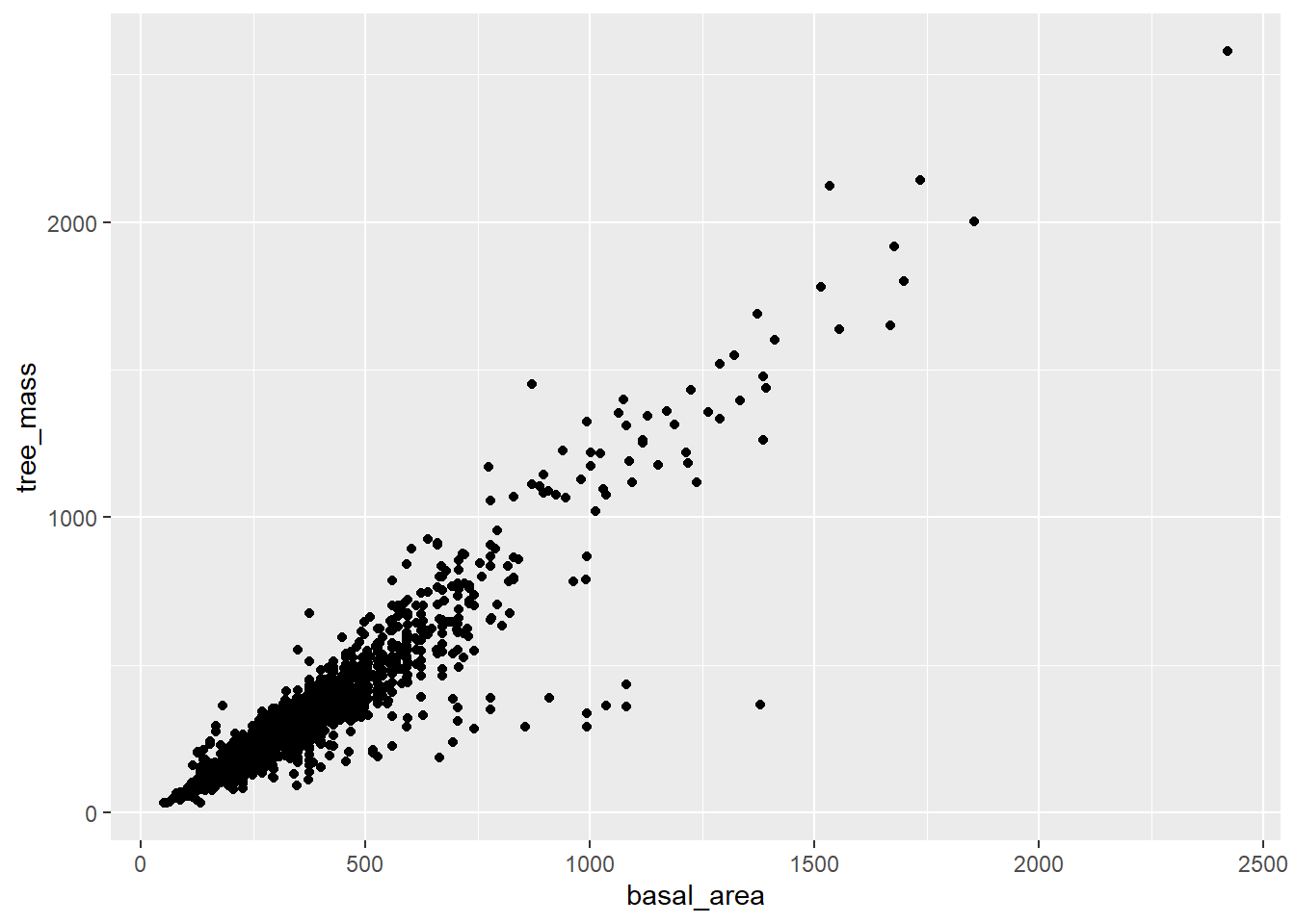
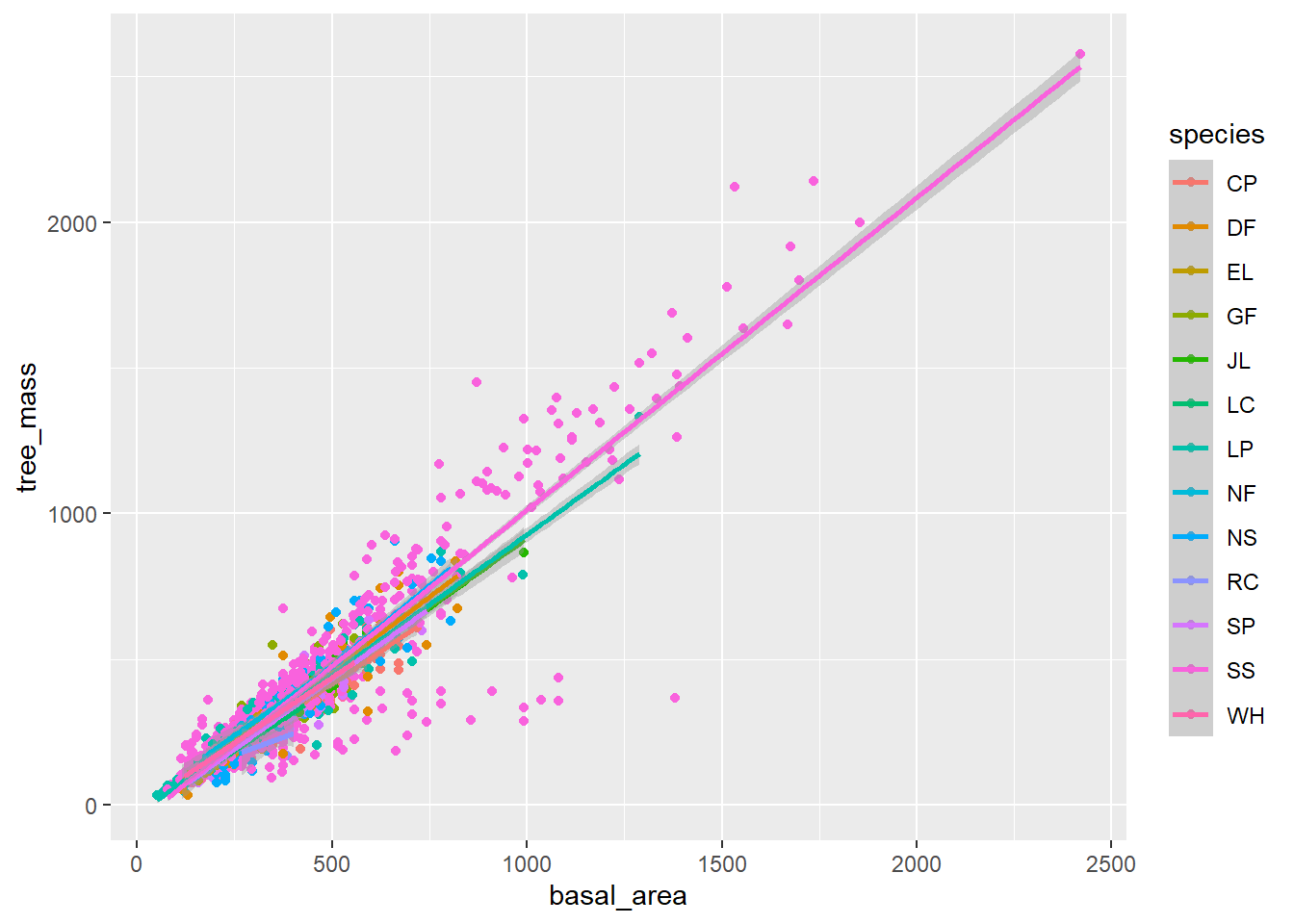
It is common practice to transfom the diameter at breast height to a cross-sectional area (\(\pi (d/2)^2\), referred to as “basal area”), as this gives a more linear relationship with volume and mass.
df$basal_area <- pi * (df$dbh/2)^2
Plot the relationship between basal area and tree mass using your own code, or that below.
Is there a reasonable linear relationship? If so, we can approximate the data with a linear model.
Bayesian Estimation of The Linear Model
The standard linear model uses the equation:
\[y = \alpha + \beta x + \epsilon\]
where in this case, \(y\) is the tree mass, \(x\) is the basal area, \(\alpha\) is the intercept, \(\beta\) is the slope, and \(\epsilon\) is the unexplained residual or “error” term. \(\beta\) expresses the change in tree mass (in kg) with a unit increase in basal area (in cm2), so has units of kg/cm2. \(\alpha\) is the hypothetical mass of a tree with zero basal area; you could interpret this as the mass of a tree just short of breast height (1.3 m). We assume \(\epsilon\) comes from a normal distribution with mean zero and standard deviation \(\sigma\).
We can estimate these model parameters in the Bayesian approach using the R package rstanarm2 with the code below. The function stan_glm uses syntax familiar to R users, with a formula argument (the same as in lm and many other related model-fitting functions). However, it uses a Markov chain Monte Carlo (MCMC) algorithm3 to estimate the parameters (instead of least squares or optimisation algorithms).
Load the libraries
Load the rstanarm library. ggeffects is used later for plotting output.
library(rstanarm)library(ggeffects)
Fit the model
The syntax below specifies the model: \(\mathrm{tree \_ mass} = \alpha + \beta \times \mathrm{basal \_ area} + \epsilon\) and the data frame to use.
m <-stan_glm(tree_mass ~ basal_area, data = df, iter =300, refresh =50)
More iterations
Set refresh to 0 to remove progress reporting during the MCMC runs. Around 1000 iterations seems to work, but we can use several thousand because this simple model is very fast.
m <-stan_glm(tree_mass ~ basal_area, data = df, iter =4000, refresh =0)
Examine the output
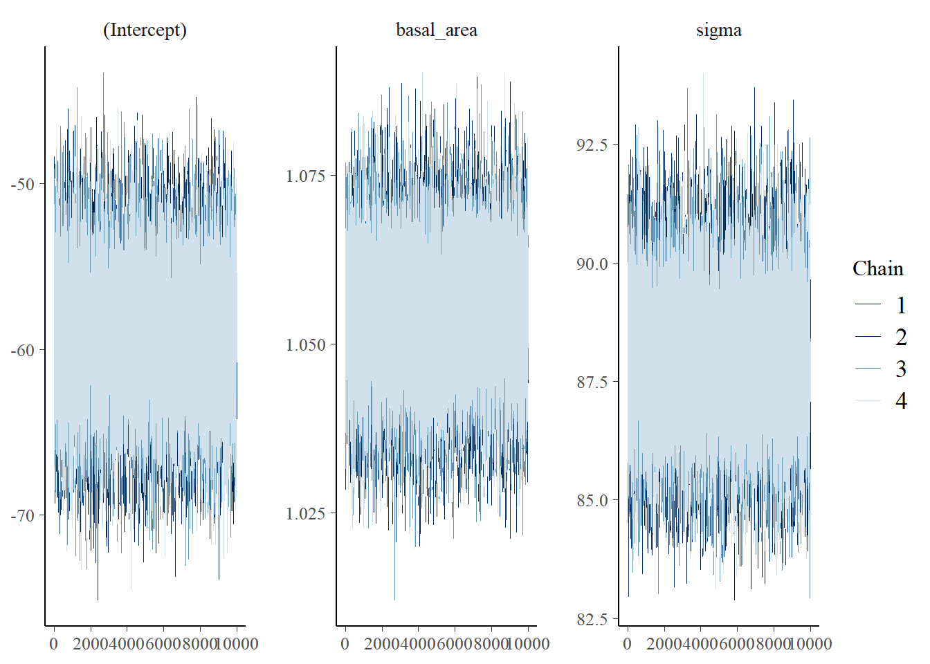
In common with other model-fitting functions in R, the \(\beta\) regression coefficient which acts as a multiplier onbasal_area is denoted simply as basal_area in the output; the \(\alpha\) coeficient is denoted as (Intercept). We can examine the trace plots from the iterations of the MCMC chains:
plot(m, "trace")
Output
and we can now get some summary output for the estimated posterior distribution:
summary(m, digits =5)
Output
Model Info:
 function:     stan_glm
 family:       gaussian [identity]
 formula:      tree_mass ~ basal_area
 algorithm:    sampling
 sample:       8000 (posterior sample size)
 priors:       see help('prior_summary')
 observations: 1901
 predictors:   2

Estimates:
              mean      sd        10%       50%       90%
(Intercept) -59.19016   3.95276 -64.25698 -59.16876 -54.13814
basal_area    1.05402   0.00933   1.04202   1.05412   1.06600
sigma        87.96231   1.44239  86.12394  87.94919  89.84348

Fit Diagnostics:
           mean      sd        10%       50%       90%
mean_PPD 324.73078   2.87349 321.04221 324.71036 328.39522

The mean_ppd is the sample average posterior predictive distribution of the outcome variable (for details see help('summary.stanreg')).

MCMC diagnostics
              mcse    Rhat    n_eff
(Intercept)   0.04512 1.00012 7675
basal_area    0.00010 1.00059 8345
sigma         0.01700 0.99964 7201
mean_PPD      0.03318 1.00006 7501
log-posterior 0.02204 1.00029 3159

For each parameter, mcse is Monte Carlo standard error, n_eff is a crude measure of effective sample size, and Rhat is the potential scale reduction factor on split chains (at convergence Rhat=1).
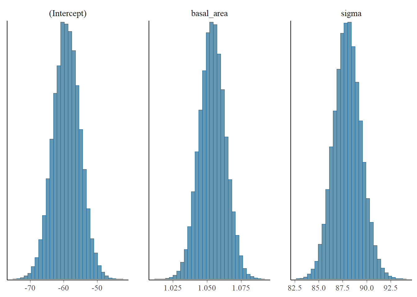
and the posterior distribution of the parameters:
plot(m, "hist")
Output
We can also explore results of the MCMC via a built-in Shiny app, launched by the launch_shinystan command:
launch_shinystan(m)
This provides a huge amount of detail - much more than you need just now, but key things are to check convergence and parameter distributions.
Examine the model fit with summary(m) and launch_shinystan(m).
Questions
Have the MCMC chains converged?
Hints
Visually inspect the trace plots for systematic changes, divergence. Is the Gelman-Rubin Statistic Rhat close to 1?
Do the parameter distributions look “sensible”?
On average, how accurate is the model?
Hints
Check the value of \(\sigma\) (sigma) in the summary output. Examine the posterior distribution of sigma.
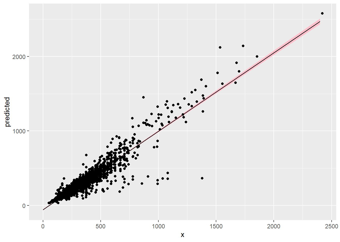
Check predictions
Plot the predictions yourself or with the code below. The ggpredict function can be used to extract the model predictions and intervals for plotting with ggplot.
Code
df_pred <-as.data.frame(ggpredict(m, terms ="basal_area [0:2400]"))p <-ggplot(df_pred, aes(x, predicted))p <- p +geom_ribbon(aes(ymin = conf.low, ymax = conf.high), fill ="pink")p <- p +geom_line()p <- p +geom_point(data = df, aes(basal_area, tree_mass))p
We can create 95 % prediction intervals by getting the appropriate quantiles of the posterior samples. Taking a mid-range basal area of 1000 cm2 (dbh ~ 35 cm):
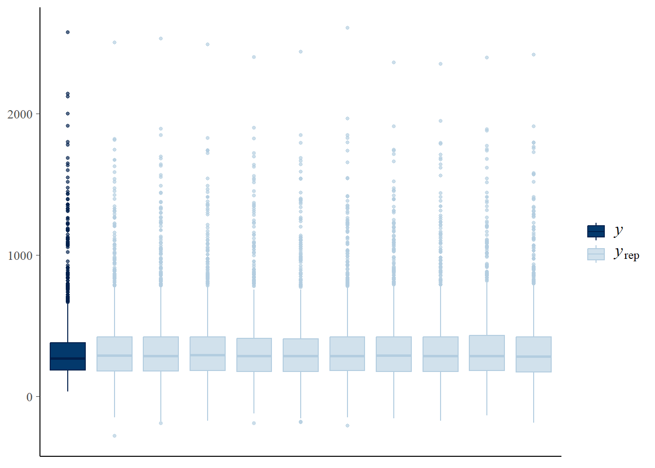
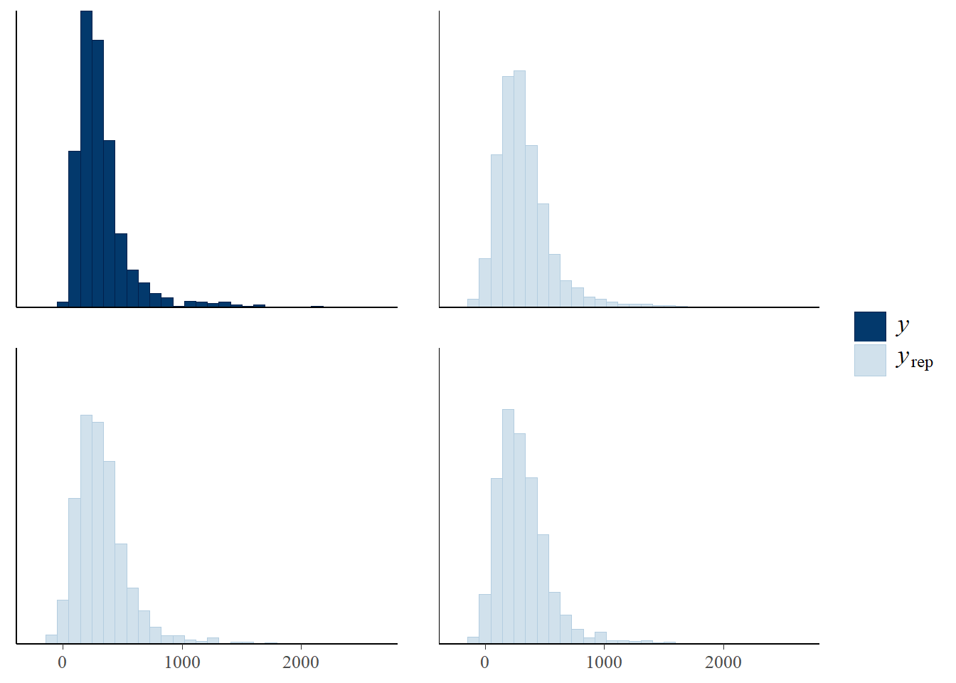
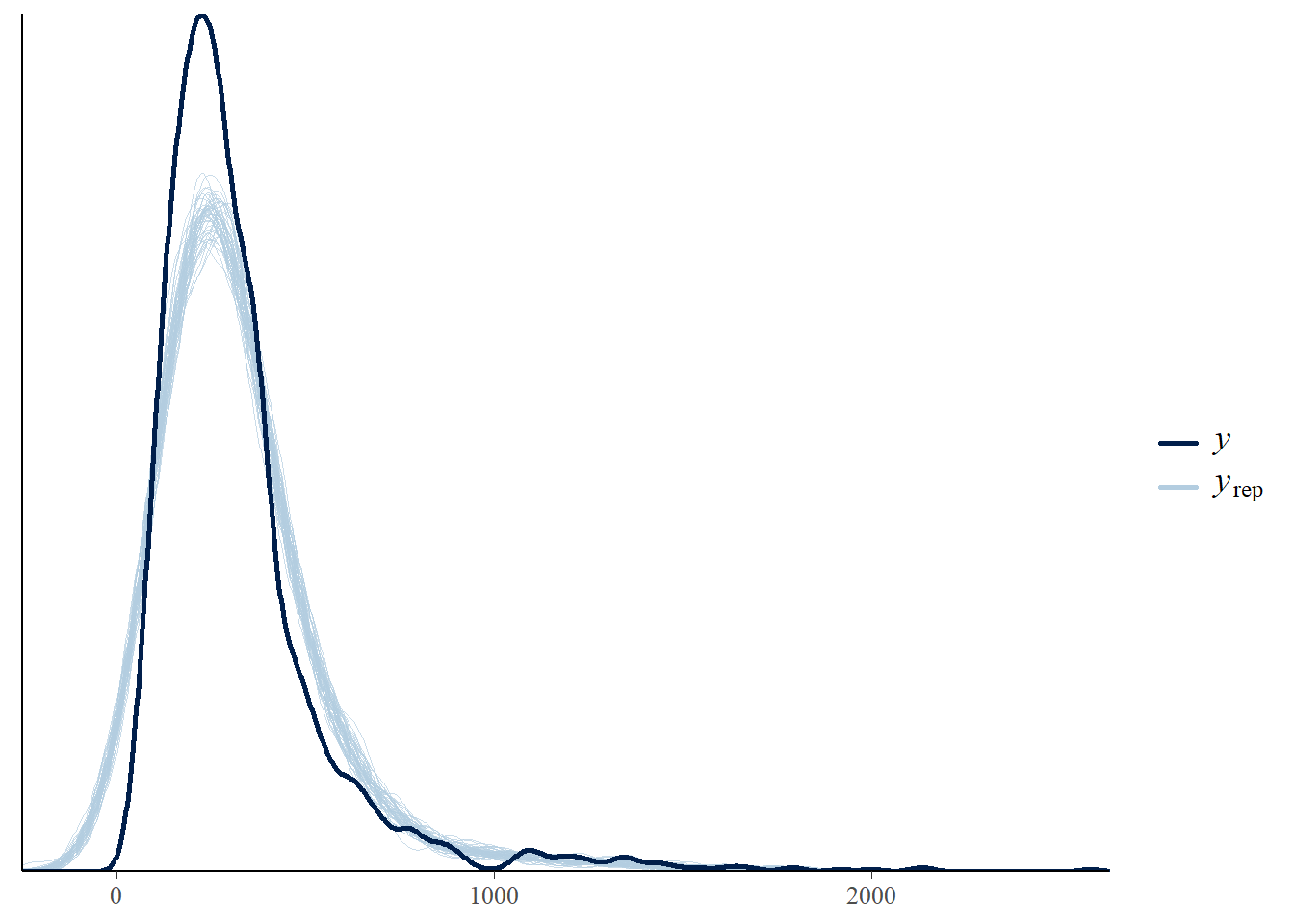
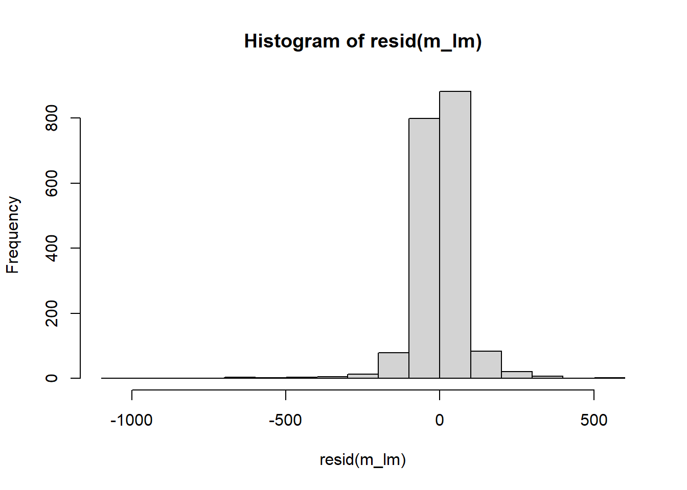
We can also check the model predictions by plotting how well they reproduce the observed data. In these plots, \(y\) is the observations, \(y_rep\) are (replicate) samples from the posterior distribution.
A Bayesian analysis considers what prior knowledge is available about the model and parameters, and combines this with the available data.
We did this using the default “weak prior”, which specifies very wide (but not uniform) distributions for all parameters. We can examine the default prior distributions for this model with the prior_PD option:
m <-stan_glm(tree_mass ~ basal_area, data = df, prior_PD =TRUE, refresh =0)
Levy, P. E., S. E. Hale, and B. C. Nicoll. 2004. “Biomass Expansion Factors and Root: Shoot Ratios for Coniferous Tree Species in Great Britain.”Forestry 77 (5): 421–30. https://doi.org/10.1093/forestry/77.5.421.
West, Geoffrey B., James H. Brown, and Brian J. Enquist. 1997. “A General Model for the Origin of Allometric Scaling Laws in Biology.”Science 276 (5309): 122–26. https://doi.org/10.1126/science.276.5309.122.
Footnotes
Biological scaling relationships apply to a wide range of morphological traits (e.g. brain size and body size), physiological traits (e.g. metabolic rate and body size in animals) and ecological traits. Some general principles seem to apply, probably because of “how essential materials are transported through space-filling fractal networks of branching tubes” (West, Brown, and Enquist 1997).↩︎
“stan” is a computer language, “ARM” is a book: “Applied Regression Modelling”.↩︎
The default alogorithm is Hamiltonian MCMC, but the details are not important just now.↩︎