here::i_am("ae/ae-05-linear.qmd")
library(here)
library(ggplot2)

df <- read.csv(url("https://raw.githubusercontent.com/NERC-CEH/beem_data/main/orings.csv"))
df <- subset(df, damage > 0)
df <- rbind(df, c(temperature = -2.5, damage = NA))Linear Modelling
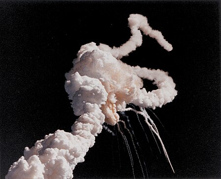
The Challenger Space Shuttle disaster
In January 1986, the Challenger Space Shuttle was due to launch. The launch programme had fallen behind schedule, and there was pressure on NASA to catch up. Unfortunately, a spell of very cold weather arrived when the launch was due, forecast to be -2.5 oC.

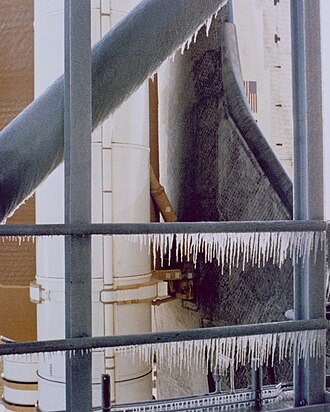
The Space Shuttle had never launched in cold weather before, and NASA engineers had to decide whether it was safe to proceed. There was concern over the “O-rings” - the rubber seals that sit within the joints of the fuel tanks. Rubber can become rigid and brittle at very low temperature; it is slow to respond when compressed, so may not form a seal within the joint.
The day before launch was due, the engineers assessed the relationship between ambient temperature and the percentage of failed O-rings where leak damage was observed in previous space shuttle missions. In this practical, we re-assess the problem they faced, and consider how a Bayesian analysis helps.
The Challenger Space Shuttle O-Ring data
First, we read and plot the data1.
Code
p <- ggplot(df, aes(x = temperature, y = damage))
p <- p + geom_point()
p <- p + stat_smooth(method = "lm", fullrange = FALSE)
p <- p + stat_smooth(method = "lm", fullrange = TRUE)
p <- p + labs(x = 'Temperature (oC)', y = 'O-Ring Leak Damage (%)')
p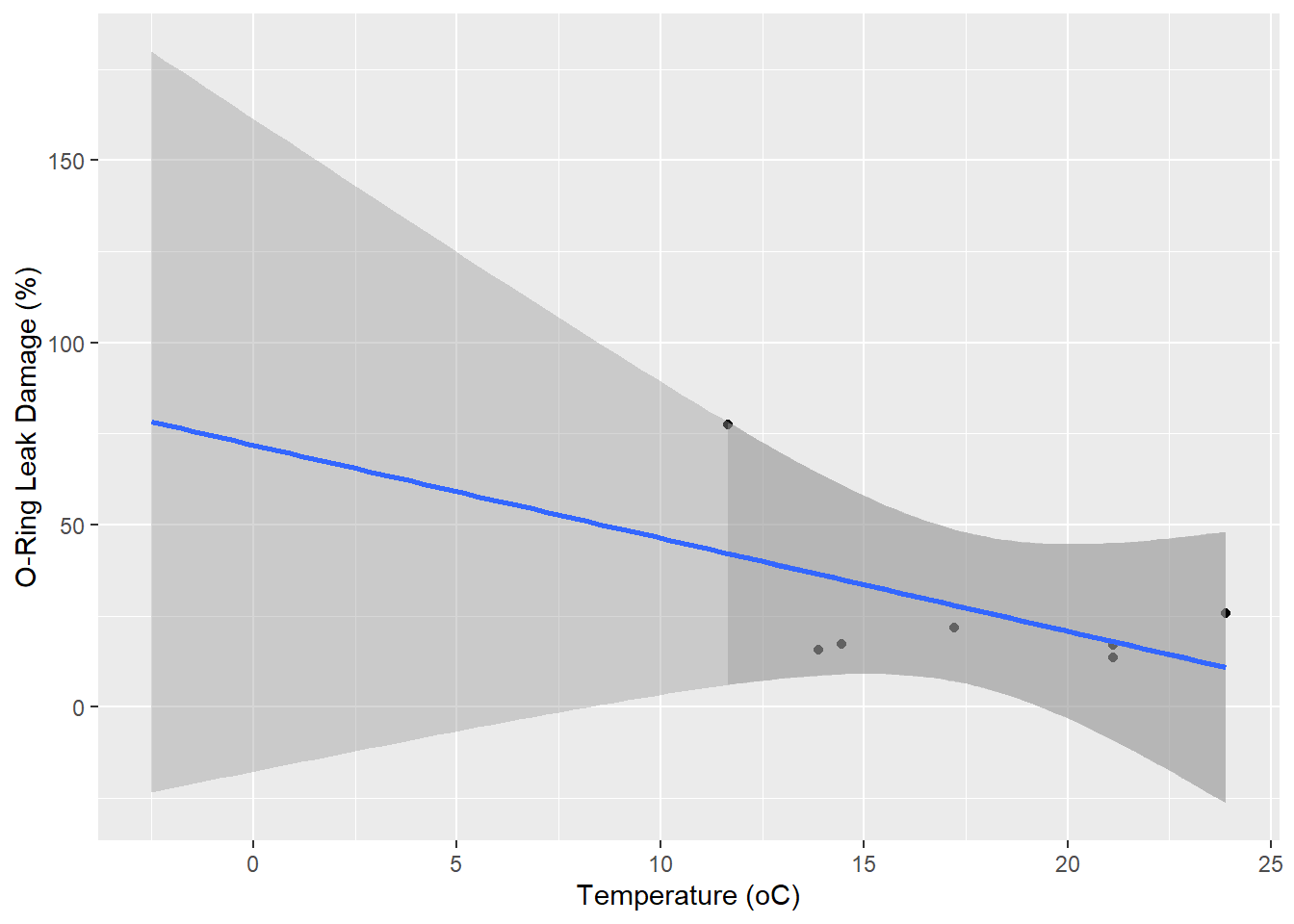
The Original (non-Bayesian) Analysis
The NASA engineers used the standard approach to linear modelling, fitting the usual equation of linear regression:
\[y = \alpha + \beta x + \epsilon\]
where in this case, \(y\) is the percentage damage, \(x\) is the temperature, \(\alpha\) is the intercept, \(\beta\) is the slope, and \(\epsilon\) is the unexplained residual or “error” term. We can fit this in R using ordinary least squares with the lm function.
m <- lm(damage ~ temperature, data = df, na.action = na.exclude)Code
summary(m)
Call:
lm(formula = damage ~ temperature, data = df, na.action = na.exclude)

Residuals:
      1       2       3       4      11      13      18
 35.375 -20.782 -17.811  -6.150  -1.026  -4.488  14.883

Coefficients:
            Estimate Std. Error t value Pr(>|t|)
(Intercept)   71.895     34.842   2.063    0.094 .
temperature   -2.553      1.924  -1.327    0.242
---
Signif. codes:  0 '***' 0.001 '**' 0.01 '*' 0.05 '.' 0.1 ' ' 1

Residual standard error: 21.36 on 5 degrees of freedom
  (1 observation deleted due to missingness)
Multiple R-squared:  0.2604,    Adjusted R-squared:  0.1125
F-statistic: 1.761 on 1 and 5 DF,  p-value: 0.2419
The slope with temperature is slightly negative (\(\beta\) = -2.55) but not significant (p = 0.242). The interpretation of this was that the data were consistent with the null hypothesis \(\beta = 0\) where there is no effect of temperature on O-ring damage. We can use the fitted model to calculate a 95% confidence interval for the predicted damage at the forecast temperature of -2.5 oC.
predict(m, newdata = data.frame(temperature = -2.5), interval = 'confidence') fit lwr upr
1 78.27606 -23.35423 179.9064This gives a very wide range, consistent with the uncertainty in the slope and the extrapolation. In the absence of a “significant” effect, the launch went ahead.
The frequentist approach is based on “letting the data speak for itself”. When the data are sparse or uncertain, this approach is inadequate.
Questions:
- Could we reject the null hypothesis that temperature has no effect on damage?
Answer
No. From the frequentist perspective, there is a probability of 0.24 that the data arose from a process in which there was no positive effect of temperature. This is greater than the usual threshold of 0.05, so we cannot reject the null hypothesis of no effect. In mathematical notation, the likelihood: \(P(data | \beta = 0) = 0.24\) - What logical fallacy was involved in the decision to launch?
Answer
They mistook the absence of evidence with evidence of absence. This is also known as the prosecuter’s fallacy, and is the confusion of two conditional probabiities. Can you put this in terms of the conditional probabiities you have learnt so far?Conditional probabiity 1
The probability of the data, given the parameters \[P(\mathrm{data} | \mathrm{no \: effect})\] \[P(y | \beta = 0)\]Conditional probabiity 2
The probability of the parameters, given the data \[P(\mathrm{no \: effect} | \mathrm{data})\] \[P(\beta = 0 | y)\]
Bayesian Analysis
A Bayesian analysis considers what prior knowledge is available about the model and parameters, and combines this with the available data. This is the approach we now take. We know from basic environmental physics (and experience) that rubber is less flexible when cold, and there is quantitative lab data available for this from materials testing. We can use such data for estimating a prior for \(\beta\). Here, we read some data from Akulichev et al (2017) and plot it.
df_lab <- read.csv(url("https://raw.githubusercontent.com/NERC-CEH/beem_data/main/rubber_rigidity.csv"))
df_lab <- subset(df_lab, temperature >= -5)

# standardise the data
df_lab$rigidity <- scale(df_lab$rigidity)
# and rescale into the damage scale
df_lab$rigidity <- df_lab$rigidity * sd(df$damage, na.rm = TRUE)Code
p <- ggplot(df_lab, aes(x = temperature, y = rigidity))
p <- p + geom_point(colour = "red")
p <- p + stat_smooth(method = "lm", fullrange = FALSE)
p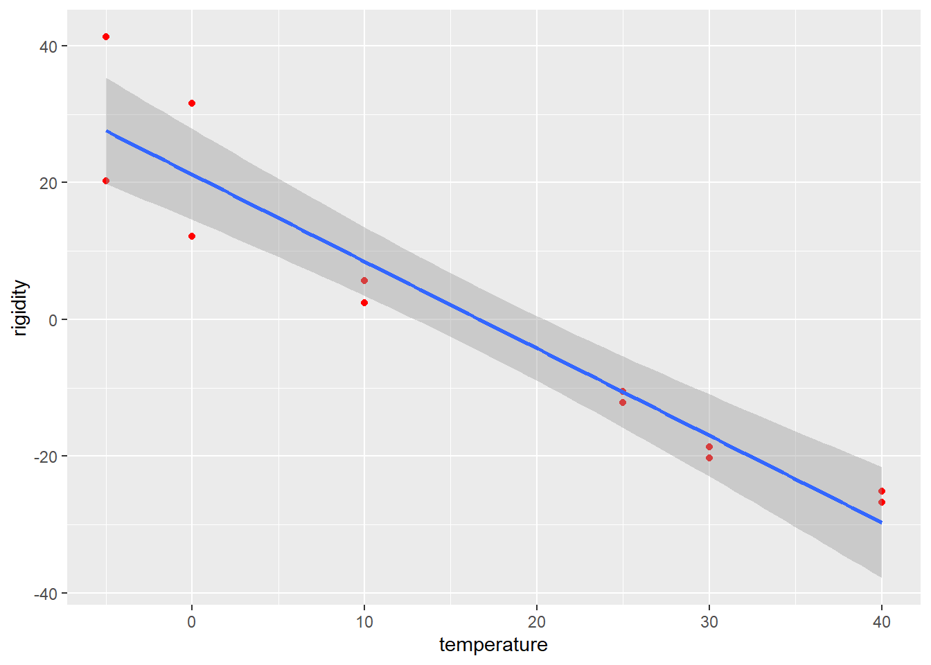
It shows the relationship betwen temperature and a measure of rigidity - the time taken for rubber O-rings to restore their original shape after being compressed. At room temperature, rubber flexes back to shape quickly; at low temperature this takes longer.
An assumption made is that the variability in damage is related to the variability in rigidity, so that we can rescale the rigidity index into damage probability percentage units2.
m <- lm(rigidity ~ temperature, data = df_lab, na.action = na.exclude)summary(m).
Code
summary(m)
Call:
lm(formula = rigidity ~ temperature, data = df_lab, na.action = na.exclude)

Residuals:
   Min     1Q Median     3Q    Max
-9.075 -3.962 -1.589  3.396 13.703

Coefficients:
            Estimate Std. Error t value Pr(>|t|)
(Intercept)  21.2187     2.9877   7.102 3.29e-05 ***
temperature  -1.2731     0.1284  -9.917 1.72e-06 ***
---
Signif. codes:  0 '***' 0.001 '**' 0.01 '*' 0.05 '.' 0.1 ' ' 1

Residual standard error: 7.224 on 10 degrees of freedom
Multiple R-squared:  0.9077,    Adjusted R-squared:  0.8985
F-statistic: 98.35 on 1 and 10 DF,  p-value: 1.715e-06
Question: 3. How strong is the relationship in the lab data?
Bayesian approach with weak prior
We can estimate the model parameters in the Bayesian approach using the R package rstanarm3 with the code below. We do this twice: once using the lab data as an informative prior, once without for comparison. We do the latter first, using the default “weak prior”, which specifies very wide (but not uniform) distributions for all parameters.
The function stan_glm has the same syntax as the lm function used earlier, but instead of least squares, it uses a Monte Carlo Markoc Chain (MCMC)algorithm4.
You can explore the output from this with a Shiny app, launched by the launch_shinystan command. This provides a huge amount of detail, but key things are to check convergence and parameter distributions. The ggpredict function extracts the model predictions and intervals for plotting with ggplot.
library(rstanarm)
library(ggeffects)
m_wp <- stan_glm(damage ~ temperature, data = df, refresh = 0)
# launch_shinystan(m_wp, ppd = FALSE)
df_wp <- ggpredict(m_wp, terms = "temperature [-5:25]")
df_wp$prior <- "weak prior"
df_pred <- as.data.frame(df_wp)summary(m_wp) and launch_shinystan(m_wp, ppd = FALSE). Plot the predictions yourself or with the code below.
Code
p <- ggplot(df_pred, aes(x, predicted))
p <- p + geom_ribbon(aes(ymin = conf.low, ymax = conf.high, fill = prior), alpha = 0.1)
p <- p + geom_line(aes(colour = prior))
p <- p + geom_point(data = df, aes(temperature, damage))
p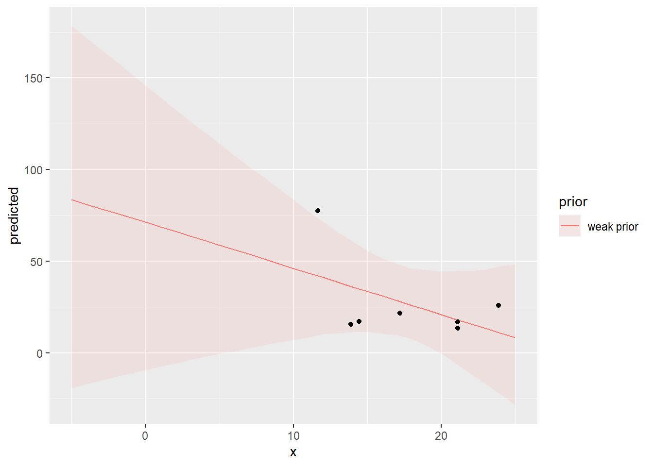
summary(m_wp)
Model Info:
 function:     stan_glm
 family:       gaussian [identity]
 formula:      damage ~ temperature
 algorithm:    sampling
 sample:       4000 (posterior sample size)
 priors:       see help('prior_summary')
 observations: 7
 predictors:   2

Estimates:
              mean   sd    10%   50%   90%
(Intercept)  71.3   40.3  24.0  71.4 118.9
temperature  -2.5    2.2  -5.1  -2.5   0.1
sigma        24.2    8.3  15.6  22.3  34.8

Fit Diagnostics:
           mean   sd   10%   50%   90%
mean_PPD 27.1   13.6 11.1  26.9  43.4

The mean_ppd is the sample average posterior predictive distribution of the outcome variable (for details see help('summary.stanreg')).

MCMC diagnostics
              mcse Rhat n_eff
(Intercept)   0.8  1.0  2415
temperature   0.0  1.0  2359
sigma         0.2  1.0  1844
mean_PPD      0.3  1.0  2639
log-posterior 0.0  1.0  1246

For each parameter, mcse is Monte Carlo standard error, n_eff is a crude measure of effective sample size, and Rhat is the potential scale reduction factor on split chains (at convergence Rhat=1).
Question: 4. How do the results compare with the least-squares regression (lm) estimates?
Bayesian approach with informative prior
Next, we use the rigidity lab data to estimate a prior distribution for \(\beta\). To characterise the response to temperature in this data, again we fit a linear model using stan_glm.
Code
m <- stan_glm(rigidity ~ temperature, data = df_lab, refresh = 0)
summary(m)
Model Info:
 function:     stan_glm
 family:       gaussian [identity]
 formula:      rigidity ~ temperature
 algorithm:    sampling
 sample:       4000 (posterior sample size)
 priors:       see help('prior_summary')
 observations: 12
 predictors:   2

Estimates:
              mean   sd   10%   50%   90%
(Intercept) 21.1    3.4 16.9  21.1  25.4
temperature -1.3    0.2 -1.4  -1.3  -1.1
sigma        8.1    2.1  5.8   7.7  10.8

Fit Diagnostics:
           mean   sd   10%   50%   90%
mean_PPD -0.1    3.4 -4.2   0.0   4.1

The mean_ppd is the sample average posterior predictive distribution of the outcome variable (for details see help('summary.stanreg')).

MCMC diagnostics
              mcse Rhat n_eff
(Intercept)   0.1  1.0  2601
temperature   0.0  1.0  2412
sigma         0.0  1.0  2217
mean_PPD      0.1  1.0  3379
log-posterior 0.0  1.0  1227

For each parameter, mcse is Monte Carlo standard error, n_eff is a crude measure of effective sample size, and Rhat is the potential scale reduction factor on split chains (at convergence Rhat=1).
# launch_shinystan(m, ppd = FALSE)We are interested in the value and uncertainty in the \(\beta\) slope coefficient, referred to as temperature in the output. If we can assume that the probability of O-ring damage is proportional to rigidity, we can use this to characterise the prior distribution for \(\beta\). The code below extracts the relevant values from the rigidity model and specifies these as the prior in the damage model. We then run the MCMC again and compare predictions when using weak and informative priors.
lab_prior <- normal(location = c(-1.3), scale = c(0.2))
m_ip <- stan_glm(damage ~ temperature, data = df, prior = lab_prior, refresh = 0)Code
df_wp <- ggpredict(m_wp, terms = "temperature [-5:25]")
df_ip <- ggpredict(m_ip, terms = "temperature [-5:25]")
df_wp$prior <- "weak prior"
df_ip$prior <- "informative prior"
df_pred <- as.data.frame(rbind(df_wp, df_ip))

p <- ggplot(df_pred, aes(x, predicted))
p <- p + geom_ribbon(aes(ymin = conf.low, ymax = conf.high, fill = prior), alpha = 0.1)
p <- p + geom_line(aes(colour = prior))
p <- p + geom_point(data = df, aes(temperature, damage))
p <- p + labs(x = 'Temperature (oC)', y = 'O-Ring Leak Damage (%)')
p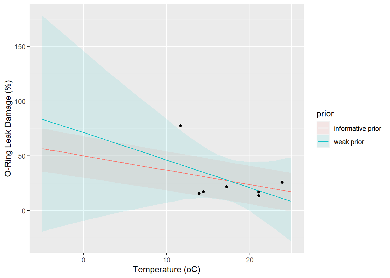
Questions:
- What effect does using an informative prior have?
- Does this better reflect our state of knowledge?
- Would this change the decision on whether to launch?
- How subjective are the decisions made about the informative prior distribution? How sensitive are the results to these?
Post-script
The seven data points shown here were really analysed by OLS regression and presented to the NASA team making the launch decision. The point is that the mindset of null-hypothesis testing led to a logical fallacy and a fatal mistake, and the Bayesian approach overcomes this, at least partially. However, the bigger mistake was that many data points were excluded because they showed no damage, and were therefore deemed not relevant. Of course, most of these occurred at warmer temperatures, so the relationship being sought in the data had already been removed. If you have time, go back to the top of the code, re-read the O-ring data in from file but exclude the line which removes the zeroes:
df <- subset(df, damage > 0)
How does this change things?
Further reading
Footnotes
There have been some minor edits to the original data for pedagogical purposes.↩︎
The rigidity index is in arbitrary units. We are effectively assuming that one standard deviation in rigidity \(\sigma_\mathrm{rigidity}\) equates to one standard deviation in damage \(\sigma_\mathrm{damage}\). This seems a reasonable assumption, but is certainly debateable. To explore the sensitivity to this, you can try different scalings between the two variables.↩︎
“stan” is a computer language, “ARM” is a book: “Applied Regression Modelling”.↩︎
The default alogorithm is Hamiltonian MCMC, but the details are not important just now.↩︎