In this practical, we are going to learn about some basic probability distributions and commands in R. We will use these to calculate probabilities under some simple examples and then apply Bayes theorem to estimate some conditional probabilities.
Some key probability distributions
These are (arguably) the most common probability distributions and the name R uses for them in brackets. Some you may know, some you may not.
Binomial (binom). This is characterised by 2 parameters - n and p, which define the number of trials and the probability of success respectively
Poisson (pois). This is characterised by 1 parameter - lambda, which specifies the mean.
Uniform (unif). This is specified by 2 parameters - min and max, denoting the lower and upper limits over which the probability density is equal.
Exponential (exp). This is specified by 1 parameter - the rate, which is equal to 1/mean.
Normal (norm). This is specified by 2 parameters- mean and sd, denoting the mean and standard deviation respectively.
Beta (beta). Specified by 2 shape parameters (\(\alpha\) and \(\beta\)), both of which are positive values, it covers the interval [0,1]. The mean is given by \(\alpha/(\alpha+\beta)\)
Gamma (gamma). Specified by 2 parameters known as the shape and scale (often denoted by \(\alpha\) and \(\sigma\) respectively. The mean of the distribution is given by \(\alpha \cdot \sigma\)
Rather than consider theoretical aspects of these distributions (which wikipedia covers reasonably well), lets use R to view them and see what they look like!
R has handy built in functions to calculate all important aspects of probability distributions, given their parameters. There are 4 key functions for every distribution:
The cumulative probabity (p), which is the probability density less than or equal to the specified value.
The probability density (d), which is the density of the probability distribution at the specified value
The quantile of the distribution (q), which returns the value for which the cumulative probability is equal to that specified. It is therefore the opposite of p.
A random draw from the distribution (r), which returns a value drawn at random from the distribution specified.
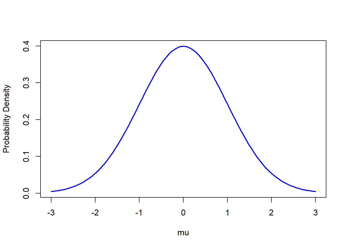
Let’s look at these more closely with a (perhaps) familiar example - the normal distribution. We all know what this look like, but what is that bell shaped curve telling us? It’s telling us the probability density for the set of values along the x axis. So let’s try and plot this.
# specify a range of values for which we are interested in the probability densitymu <-seq(-3,3,len=100)# at each value, calculate the corresponding density according to a normal distribution with mean=0, std dev=1p.dens <-dnorm(mu, mean=0, sd=1)# we can now plot this density to see the tradidional bell shaped curveplot(mu, p.dens, type="l",lwd=2, col="blue",xlab ="mu", ylab="Probability Density")
We can use the other functions in R to calculate some probabilities.
# What proportion (i.e. probability) of the data is below the mean value of 0?
pnorm(0, mean=0, sd=1)
[1] 0.5
# Let's do that the other way round. # What value is given by the 50th percentile (and therefore half the values are below it)?qnorm(0.5, mean=0, sd=1)
[1] 0
Repeat the above code for the value of 1.96 (rather than 0 in pnorm) and then vice versa in qnorm. Anything familiar?
Finally, we will consider how to draw values (or simulate observations) from a specified distribution
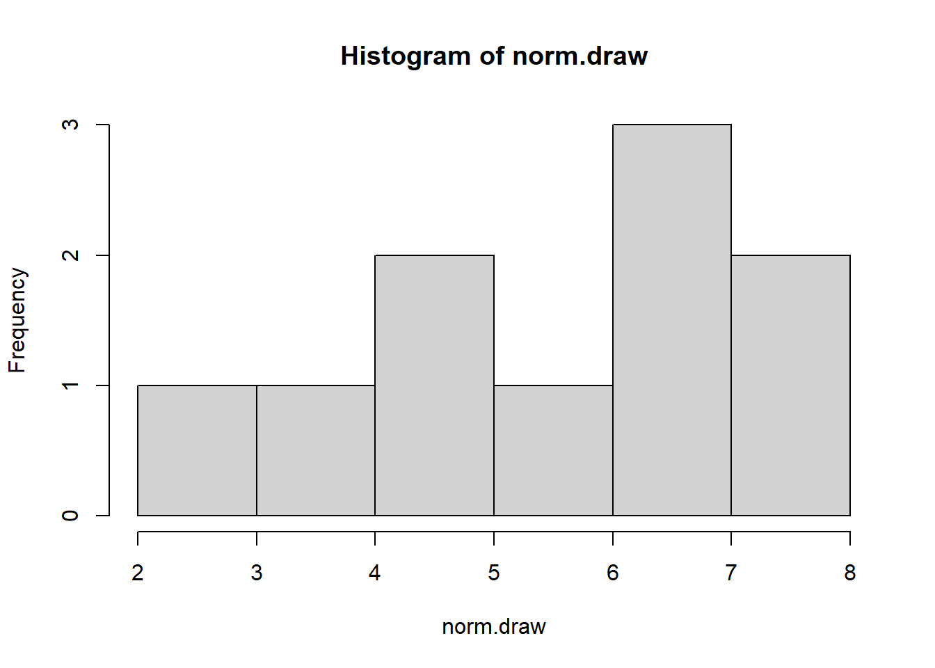
# Lets draw a value from a normal distribution with mean=5.6 and std dev=1.5norm.draw <-rnorm(1, mean=5.6, sd=1.5)# We can use the same command to draw multiple values from the same distributionnorm.draw <-rnorm(10, mean=5.6, sd=1.5)# and we can visualise this by a histogram of the datahist(norm.draw)
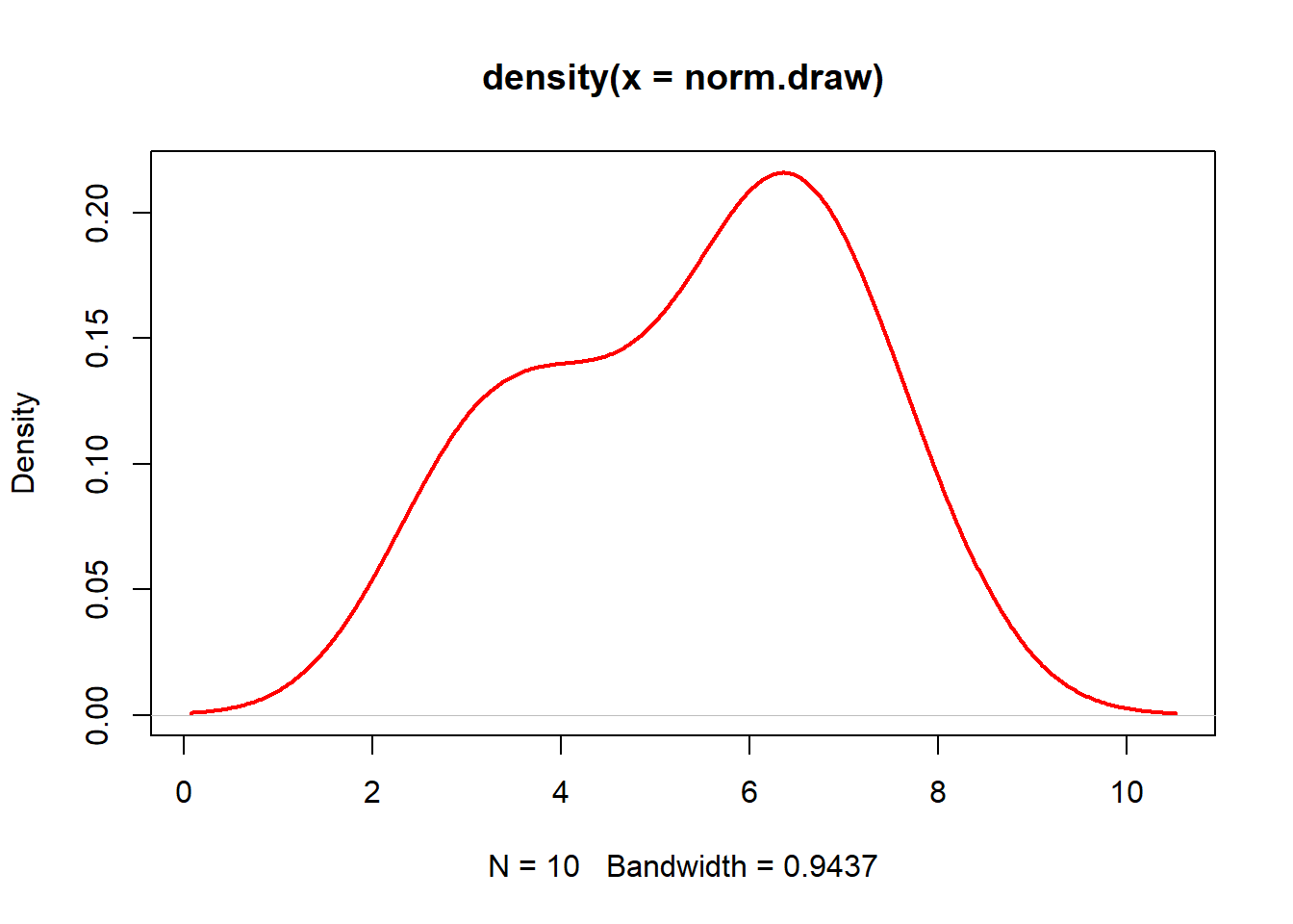
# or using a density plotplot(density(norm.draw),type="l", lwd=2, col="red")
################################################################################# TRY REPEATING THE ABOVE CODE FOR MORE THAN 10 VALUES AND SEE WHAT HAPPENS###############################################################################
Your turn
Go through the other distributions, use the “d” functions to look at shape for a given set of parameters and use the “r” functions to simulate some data
As you do this consider the shape of the distributions and any interesting properties you notice.
Conditional Probability and using Bayes’ Theorem
Assume we are interested in estimating the prevalence of ash dieback within forests across the UK, based on a sample of 50 randomly selected forests. Based on the sample ash dieback was found in 39 of the 50 forests sampled. Since the outcome is binary and we assume the forests to be independent of each other (critical assumption), we can model ash dieback prevalance with the binomial distribution.
Based on the previous exercise, we can say the parameters correspond to: n = 50, the number of forests sampled; and p is the unknown probability of ash dieback.
We have a model (binomial distribution), we have observed some data, next (as we Bayesians), we should think what sort of prior information we’d like to use for the unknown parameter p.
Think clearly about some key properties of p that the prior should represent
Would a normal distribution with mean=0 and std dev=1 be an appropriate prior? Why?
# Specify the sample sizeN <-50# The observed data represent the 39 forests in which ash dieback was detectedx <-39# We specify a value for the unknown prevalence, p, that we are interested in calculating the posterior probability forprob_guess <-0.5# Calculate the likelihood# This is given by the probability density at the given value - we know how to do this! likelihood <-dbinom(x = x, size = N, prob = prob_guess)# Calculate the prior# Again this is the probbaility density at the specified valueprior <-dunif(prob_guess, min=0, max=1)# Calculate the posterior probabilitylikelihood*prior
[1] 3.317678e-05
Repeat the above code for different values of prob_guess, saving them each time, so that you can then plot up the posterior probabilities. where this is highest provides the best guess for the true prevalance of ash dieback.
Repeat the exercise with a different choice of prior. For example a beta(2,8) or a beta(8,2) distribution. You might want to see what these look like first using what you learnt at the start of this practical.