Bayesian Basics Practical 2

Bayesian Basics

This practical contains 2 short examples that we will go through togehter in the session to further understand some of the theoretical basics of baysian approaches and also an intuitive understanding of using sampling methods to approximate posterior distributions.

Part I

On a summers’ day, I am counting the number of large white butterflies in \(T\) minutes. I assume that this count follows a Poisson distribution with mean \(\lambda T / 60\), where \(\lambda\) is unknown. i.e. our rate \(\lambda\) is the rate per hour.

I sit staring out of my window one lunchtime and I wonder if I’ll miss anything if I go for a 20min lunch break

I’m a Bayesian, so I decide that my prior on \(\lambda\) is given by an exponential distribution with mean = 5

If I observed 3 butterflies in the previous 60 mins, am I ok to go and get some lunch?

We will go through this theoretically as a class, but here lets just use what we know about distributions and plug in some guesses to build up a picture of the distribution for \(\lambda\).

#set our observation (y) as the 3 we observed in the previous hour
N_obs <- 3

#set out prior rate (which for the exponential distribution is the inverse of the mean)
prior_rate <- 1/5

#create a vector of guesses for the unknown "encounter" rate
rate_guess <- seq(0,10,len=100)

likelihood <- dpois(x = N_obs, lambda = rate_guess)
prior <- dexp(x = rate_guess, rate = prior_rate)

# Calculate the posterior probability
post_prob <- likelihood*prior

plot(rate_guess,post_prob)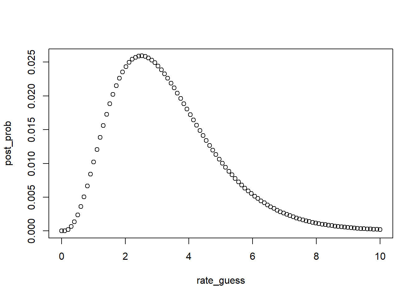

For prediction we multiply the probability of data conditional on the unknown parameter by the posterior distribution of the parameter and integrate out.

In this case we can therefore do the following:

#the likelihood of my future observation, noting that the rate has been scaled for 20min lunch, is given by 
lik_0 <- dpois(0,rate_guess/3)

#we can multiply this by the posterior distribution on the rate
pred_dens <- lik_0*post_prob

#and then sum (approximation to integrating) to get
sum(pred_dens)

[1] 0.3581407

So in this case, the probability says that I am more likely than not (probability of observing no butteflies was less than 0.5) to miss an observation if I have lunch now.

Say I had only observed 2 in the previous hour. Would I be more confident going for lunch?

This example can also be carried out entirely mathematically, which (time permitting) we will go through as a class.

Part II

In this part, we will consider the simple problem of ash dieback prevalence introduced in practical session 1b. As a reminder, we observed ash dieback in 39 of the 50 forests and are using a binomial distribution to help understand the probability of occurrence.

We will set this up, exactly as before

# Specify the sample size
N <- 50

# The observed data represent the 39 forests in which ash dieback was detected
x <- 39

# We specify a value for the unknown prevalence, p, that we are interested in calculating the posterior probability for
prob_guess <- 0.5

# Calculate the likelihood
# This is given by the probability density at the given value - we know how to do this! 
likelihood <- dbinom(x = x, size = N, prob = prob_guess)

# Calculate the prior
# Again this is the probbaility density at the specified value
prior <- dunif(prob_guess, min=0, max=1)

# Calculate the posterior probability
post_prob <- likelihood*prior

However, this time rather than guessing values of prob_guess, we want to propose values, accept or reject these based on the posterior probability and then use the density of sample points to approximate the posterior distribution.

#use our existing guess from the code above as a starter
isims = prob_guess
posts = post_prob

#suppose we want 20 samples, we set up a loop to sample until we reach 20 accepted samples
while(length(isims)<20){

  #store the current number of samples achieved
  curr.idx <- length(isims)
  
  #suggest a new proposal
  prob_guess_i <- runif(1,0,1)
  
  #run through the same posterior calculations as previous
  lik_i <- dbinom(x = x, size = N, prob = prob_guess_i)
  prior_i <- dunif(prob_guess_i, min=0, max=1)
  post_prob_i <- lik_i*prior_i

  #now only stire the result based on an improved posterior
  if(post_prob_i + rnorm(1,0,0.02)>=posts[curr.idx]){
    isims <- c(isims,prob_guess_i)
    posts <- c(posts,post_prob_i)
  }  
}  
  
#look at the historgram of the accepted proposals - this approximates our posterior density
hist(isims)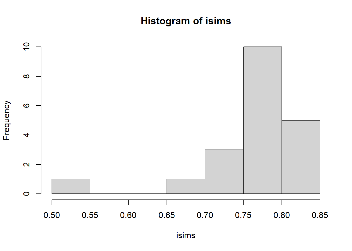

This code works fine and produces useful output, but it is incredibly slow because so many values are rejected. This is because each time we just sample from a uniform distribution. Efficiency gains are made by sampling the space more effectively!