  set.seed(123)
  n         <- 5000
  xproposed <- cbind( runif(n,0,1), runif(n,0,1) )
  plot(xproposed, asp=1)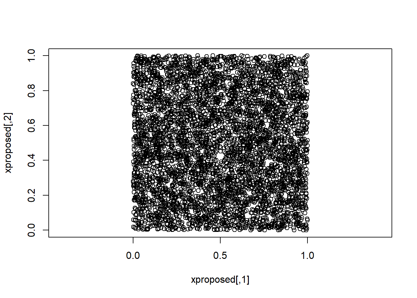
  iaccept   <- xproposed[,1]^2 + xproposed[,2]^2 < 1
  x         <- xproposed[iaccept,]
  plot(x, asp=1,main="MC-sampling")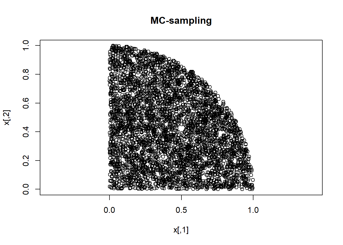
Code examples in R
This document gives a basic introduction to Markov Chain Monte Carlo sampling (MCMC) using R code examples. MCMC is a method for sampling from a probability distribution p(x). The method is completely generic, it can produce a representative sample from any kind of distribution. So p(x) can be continuous or discrete, univariate or multivariate.
The document is split into two sections demonstrations and optional further examples. The demonstrations R examples will used in the accompanying talk on MCMC as part of the course. The optional further R code examples will not be covering explicitly in the talk but have been included as useful demonstrations of the flexibility of the MCMC method.
MCMC is a specific subset of Monte Carlo sampling. We begin by demonstrating a sampling method that is MC but not MCMC.
Say we want to sample from a distribution p(x) that is bivariate, and is uniform within the overlapping area of the unit square and the unit circle. We can use MC to sample from that using the following code.
set.seed(123)
n <- 5000
xproposed <- cbind( runif(n,0,1), runif(n,0,1) )
plot(xproposed, asp=1)
iaccept <- xproposed[,1]^2 + xproposed[,2]^2 < 1
x <- xproposed[iaccept,]
plot(x, asp=1,main="MC-sampling")
Now we turn to MCMC.
MCMC can be implemented in many different ways. Here we shall only use the oldest and simplest method: the Metropolis algorithm. The method does not require you to have a formula for your distribution (such as a probability density function). Let’s use ‘p(x)’ to denote the distribution that you want to sample from. All you need to know to run the Metropolis algorithm is how to calculate the ratio of the p(x) values for any two values of x.
We begin with the same distribution that we already sampled using MC, but this time we sample using MCMC (Metropolis algorithm). So our distribution p(x) is again the bivariate uniform distribution within the overlap of the unit square and the unit circle.
pratio <- function(xa,xb) { (xa[1]^2 + xa[2]^2 < 1)  &&
                            (xa[1]>=0) && (xa[2]>=0) }
# SAMPLING FROM p(x) USING MCMC
  n      <- 500
  x      <- vector("list",n)
  x[[1]] <- c(0,0)
  for (i in 2:n) {
     xproposed <- x[[i-1]] + runif(2,-1,1)
     if ( runif(1,0,1) < pratio( xproposed, x[[i-1]]) )
        x[[i]] <- xproposed
     else
        x[[i]] <- x[[i-1]]
     end }
x <- do.call(rbind,x)
Let’s plot the Markov chain:
plot( x[ 1: 2,],xlim=c(-0.5,1.5),ylim=c(-0.5,1.5), asp=1,
      xlab="x[,1]", ylab="x[,2]") ; lines(x[1:2,],type="b")
lines(x[ 2: 3,],type="b")
lines(x[ 3: 4,],type="b")
lines(x[ 4: 5,],type="b")
lines(x[ 5: 6,],type="b")
lines(x[ 6: 7,],type="b")
lines(x[ 7: 8,],type="b")
lines(x[ 8: 9,],type="b")
lines(x[ 9:10,],type="b")
lines(x[10:11,],type="b")
lines(x[11:12,],type="b")
lines(x[12:13,],type="b")
lines(x[13:14,],type="b")
lines(x[14:15,],type="b")
lines(x[15:16,],type="b")
lines(x[16:17,],type="b")
lines(x[17:18,],type="b")
lines(x[18:19,],type="b")
lines(x[19:20,],type="b")
for(i in 21:n) {
     lines(x[(i-1):i,],type="b")
     #Sys.sleep(.09)
}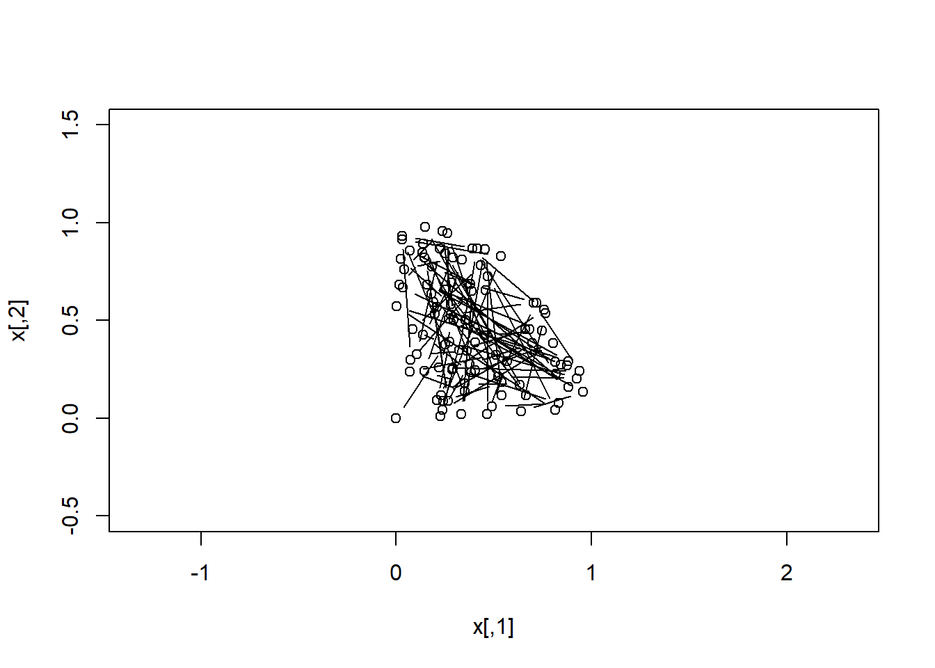
We see that the MCMC gives the same result as the MC.
Below are three examples of using MCMC (Metropolis) to sample probability distributions. These examples demonstrate the flexibility of the MCMC method to sample from very simple univariate probability distribution to more complex disjoint distributions.
We now turn to a distribution where the ratio is more complicated.
pratio <- function(xa,xb) { exp(xb^2-xa^2) }
# SAMPLING FROM p(x) USING MCMC
  n      <- 5000
  x      <- vector("list",n)
  x[[1]] <- 0
  for (i in 2:n) {
     xproposed <- x[[i-1]] + runif(1,-1,1)
     if ( runif(1,0,1) < pratio( xproposed, x[[i-1]]) )
        x[[i]] <- xproposed
     else
        x[[i]] <- x[[i-1]]
     end }
x <- do.call(rbind,x)par(mfrow=c(2,2))
plot(x,type="b")
hist(x) ; print(mean(x)) ; print(sd(x))[1] -0.059845[1] 0.7233951# In this case, R could have given the answer directly
xdirect <- rnorm(n,0,0.7)
plot(xdirect)
hist(xdirect) ; print(mean(xdirect)) ; print(sd(xdirect))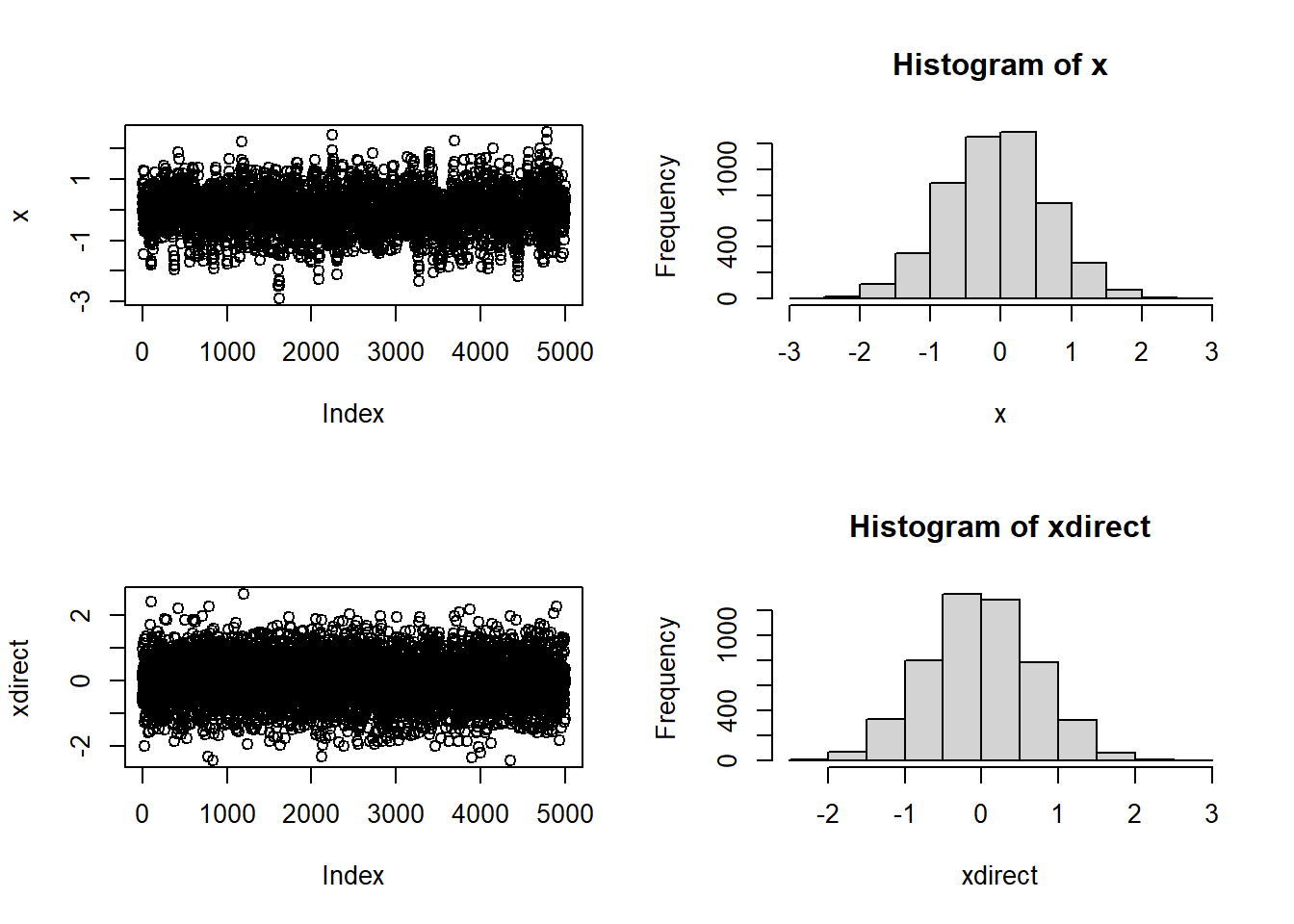
[1] -0.008340771[1] 0.7050877pratio <- function(xa,xb) { exp(xb[1]^2-xa[1]^2) * exp(xb[2]^2-xa[2]^2) }
# SAMPLING FROM p(x) USING MCMC
n <- 2000
x <- vector("list",n)
x[[1]] <- c(0,0)
for (i in 2:n) {
xproposed <- x[[i-1]] + runif(2,-1,1)
if ( runif(1,0,1) < pratio( xproposed, x[[i-1]]) )
x[[i]] <- xproposed
else
x[[i]] <- x[[i-1]]
end }
x <- do.call(rbind,x)par( mfrow=c(1,2) )
plot(x,asp=1,type="b")
# In this case too, R could have given the answer directly
xdirect <- MASS::mvrnorm( n, mu=c(0,0), Sigma=diag(c(0.5,0.5)) )
plot(xdirect,asp=1)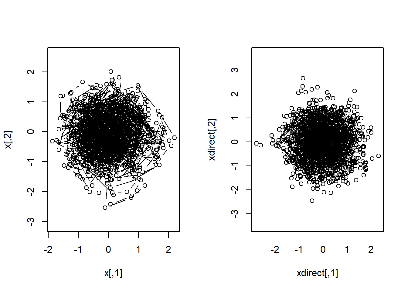
We now show that MCMC can sample from multimodal distributions, even when the modal regions are separated by a region of zero-probability.
pratio <- function(xa,xb) {  (xa[1]   ^2 +  xa[2]     ^2 < 1  ) ||
                            ((xa[1]-2)^2 + (xa[2]-0.5)^2 < 0.5)    }
# SAMPLING FROM p(x) USING MCMC
  n      <- 2000
  x      <- vector("list",n)
  x[[1]] <- c(0,0)
  for (i in 2:n) {
     xproposed <- x[[i-1]] + runif(2,-1,1)
     if ( runif(1,0,1) < pratio( xproposed, x[[i-1]]) )
        x[[i]] <- xproposed
     else
        x[[i]] <- x[[i-1]]
     end }
x <- do.call(rbind,x)par( mfrow=c(1,1) )
plot(x[1:2,],xlim=c(-1,3),ylim=c(-1,1.5),asp=1) ; lines(x[1:2,],type="b")
for(i in 3:n) { lines(x[(i-1):i,],type="b",lty=3) }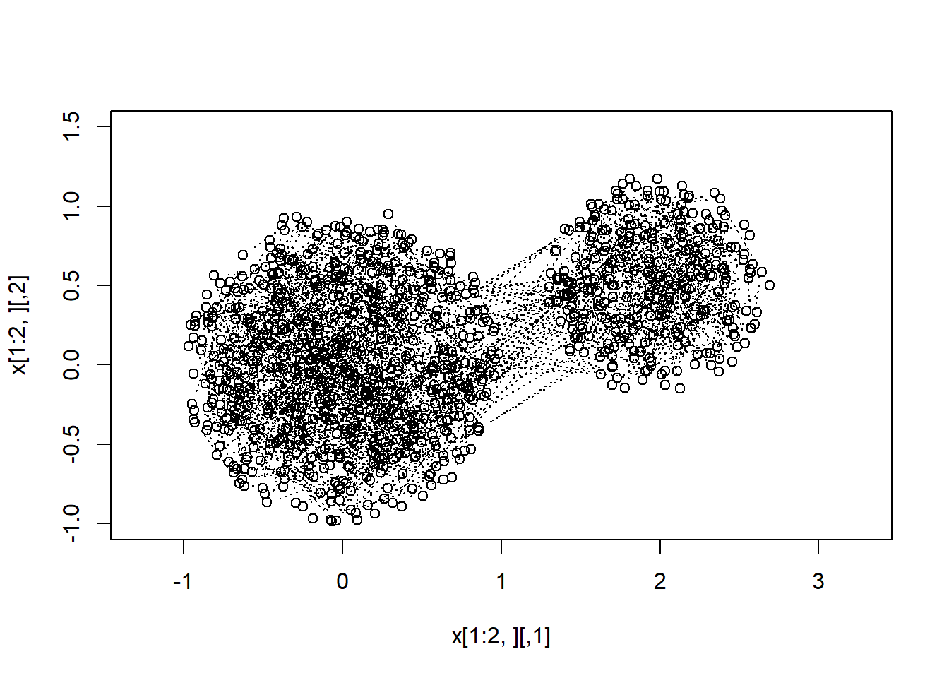
plot(x,xlim=c(-1,3),ylim=c(-1,1.5),asp=1)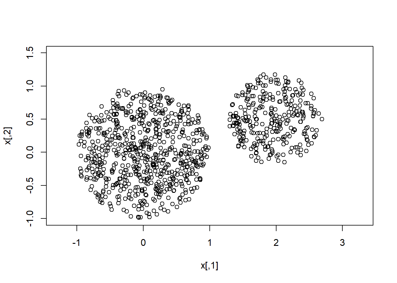
``