n = (1+1/kappa)*(sigma_s*(qnorm(1 - alpha/2) + qnorm(1-beta))/d_true)^2Measurements and Uncertainty
Bayesian Methods for Ecological and Environmental Modelling
In this practical, we will calculate the false discovery rate for a number of experimental scenarios. This involves estimating or choosing reasonable values for:
- the magnitude of the effect we are trying to detect \(d\);
- the variability \(\sigma\) in the population or samples used to estimate \(d\);
- sample size \(n\);
- threshold probability for the false positive rate \(p\) value aka. \(\alpha\) or Type I error rate;
- threshold probability for the false negative rate \(\beta\) aka. Type II error rate or statistical power (\(1 - \beta\)).
Given any four of the above, we can calculate the fifth.
As an example, we will consider the detection of change in soil carbon shown in the lecture. The variable of interest is the soil carbon stock (in kg C/m2), and we can stick to the simple case of detecting a change in the mean between two time points.
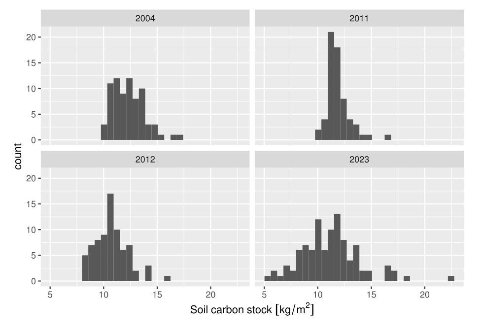
We will denote the mean soil carbon stock at time 1 and time 2 as \(\mu_{t1}\) and \(\mu_{t2}\), denoted mu_t1 and mu_t2 in the code. We are interested in the difference \(d = \mu_{t1} - \mu_{t2}\), d_true in the code. Suppose the true value of this is 0.5 kg C/m2. How many samples would be need to detect this reliably? \(\kappa\) (kappa) is the ratio of the number of samples \(n\) at time 2 cf. time 1; we can assume this equals 1 as they stay roughly similar.
We estimate the variability as the sample standard deviation \(\sigma_s\) (sigma_s) (as our proxy for the population variability). From the data, this is around 2 kg C/m2 (though much bigger in 2023).
We set the standard threshold probabilities for the false positive rate (\(\alpha\) or \(p\) value = 0.05) and the statistical power (\(1 - \beta\) = 0.8).
We can then calculate the number of samples needed to detect a change of magnitude \(d\) in a population with variability \(\sigma_s\) with probability \(\alpha\) and power \(1-\beta\) as:
which assumes a normal distribution. Run the code below which implements the power analysis outlined above.
# Set a seed for reproducibility of random numbers
set.seed(586)

mu_t1 = 10
d_true <- 0.5 # the supposed true difference
mu_t2 = mu_t1 + d_true
kappa = 1
sigma_s = 2 # spatial var in samples from the same survey
alpha = 0.05
beta = 0.20
(n = (1+1/kappa)*(sigma_s*(qnorm(1 - alpha/2) + qnorm(1-beta))/d_true)^2)
[1] 251.1642ceiling(n) # rounds up to an integer[1] 252There is also a fairly reliable rule-of-thumb formula for two-sided tests like this.
# rule of thumb for n
16 * sigma_s^2 / d_true^2
[1] 256We therefore need around 252 samples to detect this change reliably. In fact, our sample size was often around 80. We can calculate how much this reduces the statistical power as follows.
n = 80 # lower true sample size
z <- d_true / (sigma_s*sqrt((1+1/kappa)/n))
(power_actual = pnorm(z  - qnorm(1 - alpha / 2))
              + pnorm(-z - qnorm(1 - alpha / 2)))
[1] 0.3526081We can calculate the expected false discovery rate based on the actual statistical power of our experiment, if we assume a prior probability for a change of magnitude \(d\). This is a bit subjective. There was no consistent change in management at this site over the last 20 years, so there is no particular reason to expect a change in soil carbon, so the probability of a change of this magnitude is fairly unlikely. However, there may be effects of climate change or more subtle changes in management, so we should not rule it out. A 10 or 20% probability seems reasonable.
beta_actual <- 1 - power_actual
P_H1 <- 0.2
power_naive <- 0.8
# naive expected fdr
(fdr <- 1 - (P_H1 * power_naive)  / (P_H1 * power_naive  + alpha * (1 - P_H1)))
[1] 0.2# actual fdr
(fdr <- 1 - (P_H1 * power_actual) / (P_H1 * power_actual + alpha * (1 - P_H1)))[1] 0.3619201This gives a false discovery rate of 36.2 %. Taking the more conservative prior:
P_H1 <- 0.1
# actual fdr
(fdr <- 1 - (P_H1 * power_actual) / (P_H1 * power_actual + alpha * (1 - P_H1)))
[1] 0.5606722we get a much higher rate of 56.1 %.
An equally serious problem is the likely presence of systematic biases between surveys. The effect of this is best examined using simulation. First, we declare a number of simulations and some vectors to store the results.
n_sims <- 10000
# prob of false pos given difference
v_p_h1 <- vector(mode = "numeric", length = n_sims)
# prob of true pos given no difference
v_p_h0 <- vector(mode = "numeric", length = n_sims)
We then simulate n_sim simulations, in each of which we generate:
- \(n\) values of soil carbon stock at time 1 \(y_{t1}\)
y_t1 - a bias which influences the values observed at time 2, which is normally distributed, is on average zero, but has standard deviation \(\sigma_b\)
- \(n\) values of soil carbon stock at time 2 \(y_{t2}\)
y_t2_h0under the hypothesis of no change (\(mu_{t1} = mu_{t2}; d = 0\)) - \(n\) values of soil carbon stock at time 2 \(y_{t2}\)
y_t2_h1under the hypothesis of change (\(mu_{t2} = mu_{t1} + d\)) - in both cases, we carry out a t-test and store the p-value returned (the apparent probability that the difference between samples arose without any difference in the means at t1 and t2).
sigma_b = 0   # check we get the same results as above with zero bias

for (i in seq_along(1:n_sims)) {
  y_t1  <- rnorm(n, mu_t1, sigma_s)
  bias <- rnorm(1, 0, sigma_b)
  y_t2_h0  <- rnorm(n, mu_t1 + bias, sigma_s)
  y_t2_h1  <- rnorm(n, mu_t2 + bias, sigma_s)
  v_p_h1[i] <- t.test(y_t1 - y_t2_h1)$p.value
  v_p_h0[i] <- t.test(y_t1 - y_t2_h0)$p.value
}
We can calculate the power empirically as the fraction of simulations where the t-test returned a positive result when the difference was present. Similarily, we can calculate the p-value (\(\alpha\)) empirically as the fraction of simulations where the t-test returned a positive result when the difference was not present.
(power_actual <- sum((v_p_h1 < alpha) / n_sims))[1] 0.3438(alpha_actual <- sum((v_p_h0 < alpha) / n_sims))[1] 0.053# hist(v_p_h1); hist(v_p_h0)We can use these values to calculate the false discovery rate, incorporating the effects of bias between surveys.
(beta_actual <- 1 - power_actual)[1] 0.6562P_H1 <- 0.1
power_naive <- 0.8
# naive expected fdr
(fdr <- 1 - (P_H1 * power_naive) / (P_H1 * power_naive + alpha * (1 - P_H1)))[1] 0.36# actual fdr
(fdr <- 1 - (P_H1 * power_actual) / (P_H1 * power_actual + alpha_actual * (1 - P_H1)))[1] 0.5811404Having convinced ourselves that this gives the same value of power as above when the bias is zero, we can add in a bias term and see its effect. A value of sigma_b = 0.5 looks plausible (probably an under-estimate), given the difference between the means in 2011 and 2012 of 1.2 kg C/m2, which is too short a time for any real change to occur.
sigma_b = 0.5 # typical bias between survey results

for (i in seq_along(1:n_sims)) {
  y_t1  <- rnorm(n, mu_t1, sigma_s)
  bias <- rnorm(1, 0, sigma_b)
  y_t2_h0  <- rnorm(n, mu_t1 + bias, sigma_s)
  y_t2_h1  <- rnorm(n, mu_t2 + bias, sigma_s)
  v_p_h1[i] <- t.test(y_t1 - y_t2_h1)$p.value
  v_p_h0[i] <- t.test(y_t1 - y_t2_h0)$p.value
}
We can calculate the power empirically as the fraction of simulations where the t-test returned a positive result when the difference was present. Similarily, we can calculate the p-value (\(\alpha\)) empirically as the fraction of simulations where the t-test returned a positive result when the difference was not present.
(power_actual <- sum((v_p_h1 < alpha) / n_sims))[1] 0.4329(alpha_actual <- sum((v_p_h0 < alpha) / n_sims))[1] 0.299# hist(v_p_h1); hist(v_p_h0)We can use these values to calculate the false discovery rate, incorporating the effects of bias between surveys.
(beta_actual <- 1 - power_actual)[1] 0.5671P_H1 <- 0.1
power_naive <- 0.8
# naive expected fdr
(fdr <- 1 - (P_H1 * power_naive) / (P_H1 * power_naive + alpha * (1 - P_H1)))[1] 0.36# actual fdr
(fdr <- 1 - (P_H1 * power_actual) / (P_H1 * power_actual + alpha_actual * (1 - P_H1)))[1] 0.8614232With potential biases between surveys, the expected false discovery rate becomes extremely high: 86%. In experiments similar to this, if “significant” differences are found with reported p-values of < 0.05, can you take the results at face value? In this instance, we did not need to propagate any additional uncertainty to illustrate the point, because the spatial variability between samples was large. In many cases, the uncertainty is present but not propagated, so not apparent in the results.
Exercises:
- Vary the sample number, the variability and the prior probability values. How do these affect the false discovery rate? Are the effects linear?
- If you have any experiments in your own work, calculate the statistical power of the current design. Do you have a big enough sample size to see the expected effect? What is a likely false discovery rate?