As trees grow, they grow both horizontally in girth (and diameter) and vertically in height. But as trees age and gain size, the change (growth rate) in height declines; the relationship is non-linear (e.g. Banin et al. 2012). This is thought to happen because as trees gain height they become less limited in light, but more limited by other growth resources (water, nutrients…) and may put more energy into reproductive processes. There are remarkable similarities in the nature of these non-linear relationships (so called ‘rules of ecology’), yet they still vary across sites and across species. These grouping variables add ‘structure’ to our data i.e. these grouping create non-independence.
We will use the relationships between height and diameter within the UK tree dataset to explore the application of hierarchical models in rstanarm.
Explore the data
Load the “trees.csv” data we have already been using.
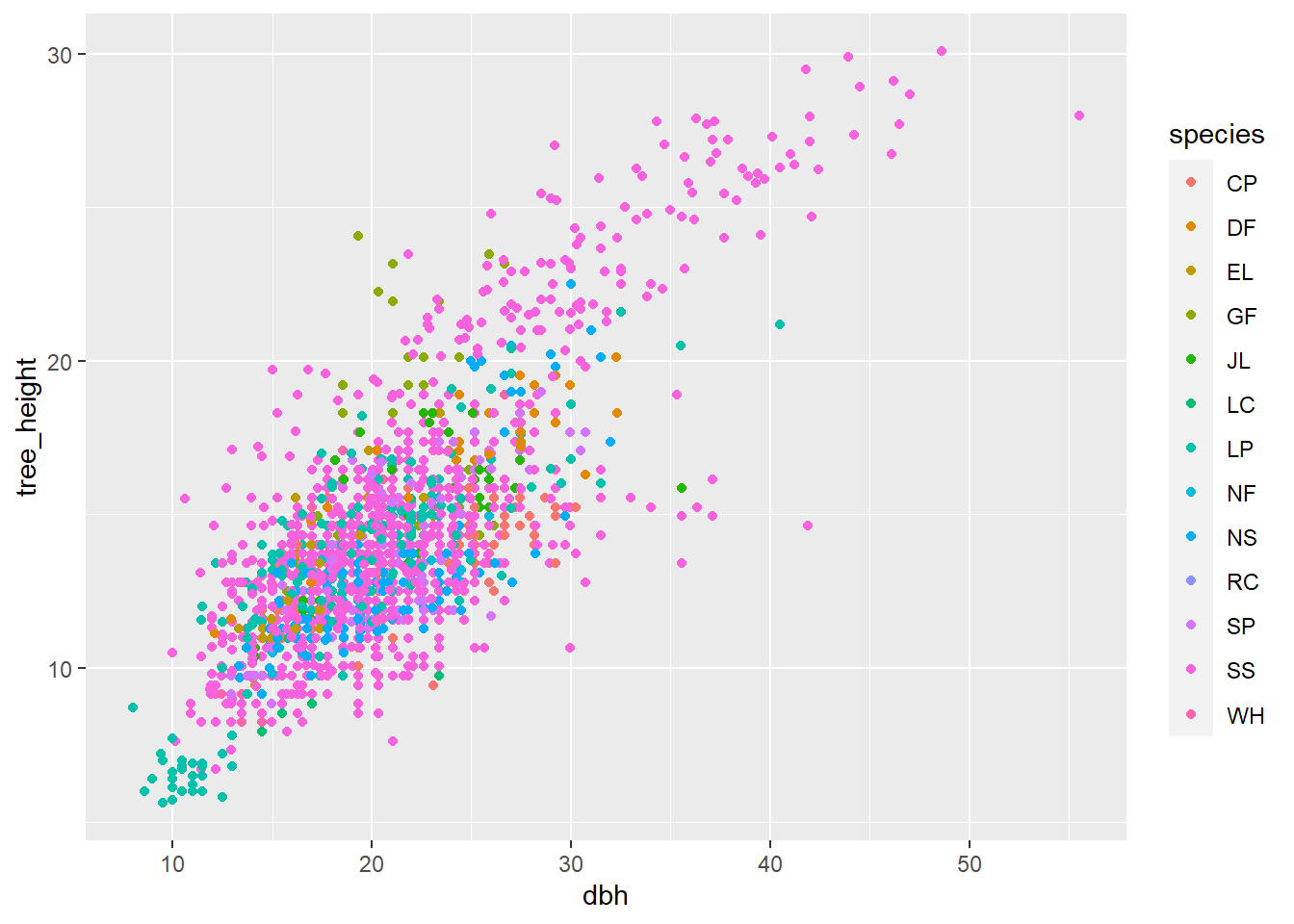
As usual, the best first step of an analysis is to get a feel for the data by plotting. We will first plot tree height against diameter (diameter at breast height; DBH), with points coloured according to the different species in the dataset. What do you observe about this plot?
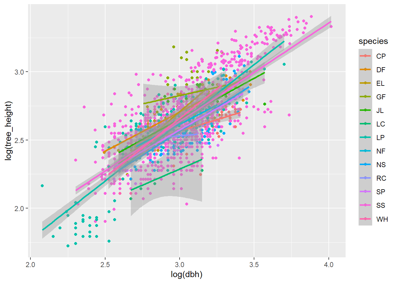
Next, we will natural-log transform both the variables of tree_height and dbh. This transforms a non-linear Power law function y = aX^b to a linear function (log(y) = a + b*(logX)). What do you observe now?
Warning: package 'ggplot2' was built under R version 4.4.3
# Plot the raw datap <-ggplot(df, aes(dbh, tree_height, colour = species))p <- p +geom_point()p
# Now natural-log transform the height and diameter at breast height (DBH)p <-ggplot(df, aes(log(dbh), log(tree_height), colour = species))p <- p +geom_point()p <- p +stat_smooth(method ="lm")p
`geom_smooth()` using formula = 'y ~ x'
The natural-log transformation will not always be the best for a non-linear relationship (for example, if your relationship exhibits an asymptote), but this is good enough for now!
The package rstanarm uses the formulation from the lme4 package, which can be used for hierarchical models using a maximum likelihood approach. Linear mixed-effects models use the function ‘lmer’ and non-linear models use the ‘nlmer’ function in the lme4 package. Before we move to the Bayesian formulation in rstanarm, let’s explore a simple model using lme4. (If this package is not familiar, we could easily dedicate a whole training session to this! But we will focus on the essential elements for now).
Creating a model using lme4
Here we will model the relationship between tree height and diameter using lme4 using the function lmer. As above, we take the log of both variables so that the relationship is linear. Much of this code will look familiar, as compared with a linear regression (lm). Here, we have an additional term which specifies how the grouping variable ‘species’ will be used in the model. In the first model (m1_lme) below, we have specified that the intercept of the height-diameter relationship varies by the group term Species using (1|species). The second model formulation allows both the intercept and slope to vary by group (diam|species). In each case, the intercepts and slopes for each species are a deviations from the parameter estimates for the intercept and slope for the whole dataset (the fixed effects), and these represent a population from a random distribution.
## Assess Tree Height and Diameter Allometric relationship using mixed effects model with lme4 packagelibrary(lme4)
Warning: package 'lme4' was built under R version 4.4.3
Linear mixed model fit by REML ['lmerMod']
Formula: height ~ diam + (1 | species)
   Data: df

REML criterion at convergence: -1527.4

Scaled residuals:
    Min      1Q  Median      3Q     Max
-3.9978 -0.6109  0.0439  0.6544  3.5501

Random effects:
 Groups   Name        Variance Std.Dev.
 species  (Intercept) 0.008072 0.08984
 Residual             0.025564 0.15989
Number of obs: 1901, groups:  species, 13

Fixed effects:
            Estimate Std. Error t value
(Intercept)  0.44100    0.05137   8.584
diam         0.72257    0.01473  49.041

Correlation of Fixed Effects:
     (Intr)
diam -0.860
ranef(m1_lme)
$species
    (Intercept)
CP -0.065595914
DF  0.074487937
EL  0.062835193
GF  0.163073601
JL  0.037563658
LC -0.181808088
LP  0.003878361
NF  0.006101305
NS -0.044023529
RC -0.082740006
SP -0.037135707
SS  0.026345056
WH  0.037018135

with conditional variances for "species"
Linear mixed model fit by REML ['lmerMod']
Formula: height ~ diam + (diam | species)
   Data: df

REML criterion at convergence: -1551.3

Scaled residuals:
    Min      1Q  Median      3Q     Max
-4.0397 -0.6159  0.0329  0.6479  3.5857

Random effects:
 Groups   Name        Variance Std.Dev. Corr
 species  (Intercept) 0.26186  0.5117
          diam        0.02559  0.1600   -0.98
 Residual             0.02503  0.1582
Number of obs: 1901, groups:  species, 13

Fixed effects:
            Estimate Std. Error t value
(Intercept)  0.63809    0.17749   3.595
diam         0.65920    0.05674  11.618

Correlation of Fixed Effects:
     (Intr)
diam -0.988
As we expected from the plotting, the relationships between tree_height and dbh are ‘shifted’ along the y-axis according to species. Let’s first proceed with our simpler model in rstanarm. Here, we run it using the function glmer (generalised linear mixed effects model) where we explicitly specify the family as Gaussian (Normal) - we could also run it using lmer in this case. We will return to more examples with generalised linear models later.
We can see that there are lots of similarities between the lmer models above and the stan_glmer model below, but we also add in some extra arguments to prescribe how our Bayesian analysis is run - notice the chains and iter (iterations) arguments. As these numbers get higher, the model takes longer to run, and you might want to check things are behaving before you set it off on lots of iterations. Let’s start small-ish. If these samples are inadequate and the chains are not converging you will get some useful warnings about effective sample size and R-hat (https://mc-stan.org/rstanarm/articles/rstanarm.html). If chains have not mixed well (so that between- and within-chain estimates do not agree), R-hat is larger than 1.
## Re-run using rstanarmlibrary(rstanarm)
Warning: package 'rstanarm' was built under R version 4.4.3
Loading required package: Rcpp
Warning: package 'Rcpp' was built under R version 4.4.3
This is rstanarm version 2.32.1
- See https://mc-stan.org/rstanarm/articles/priors for changes to default priors!
- Default priors may change, so it's safest to specify priors, even if equivalent to the defaults.
- For execution on a local, multicore CPU with excess RAM we recommend calling
options(mc.cores = parallel::detectCores())
height <-log(df$tree_height)diam <-log(df$dbh)m1_stan <-stan_glmer(height ~ diam + (1|species), data = df, family =gaussian(link ="identity"), chains =2,iter =500, seed =12345)
Warning: Bulk Effective Samples Size (ESS) is too low, indicating posterior means and medians may be unreliable.
Running the chains for more iterations may help. See
https://mc-stan.org/misc/warnings.html#bulk-ess
Warning: Tail Effective Samples Size (ESS) is too low, indicating posterior variances and tail quantiles may be unreliable.
Running the chains for more iterations may help. See
https://mc-stan.org/misc/warnings.html#tail-ess
## try editing chains and iterations and look at warnings.
m1_stan <-stan_glmer(height ~ diam + (1|species), data = df, family =gaussian(link ="identity"), chains =4,iter =2500, seed =12345)
In the code chunk above, we have not explicitly stated our priors, which means rstanarm has used the defaults. There is some really useful information about how these defaults are chosen in this vignette: https://mc-stan.org/rstanarm/articles/priors.html, and on the priors for the covariance matrix (https://mc-stan.org/rstanarm/articles/glmer.html#priors-on-covariance-matrices-1). They are intended to be weakly informative; vague but without allowing odd behaviour in the model. Let’s take a look at what these defaults are for our model.
Notice we have the same priors as for the linear regression model - for the intercept, slope coefficient, auxiliary (sigma) and we also have the prior for the covariance matrix, which relates to our random effect term (species).
To explicitly state our priors, we could write the model formula as:
The Bayesian uncertainty interval indicates we believe after seeing the data that there is 0.950�probability that�the slope parameter for log(DBH) (or diam)�is between�the lower bound ci95[1,1]�and upper bound�ci95[1,2] - a convenient interpretation for the parameters of interest as we heard on day one!
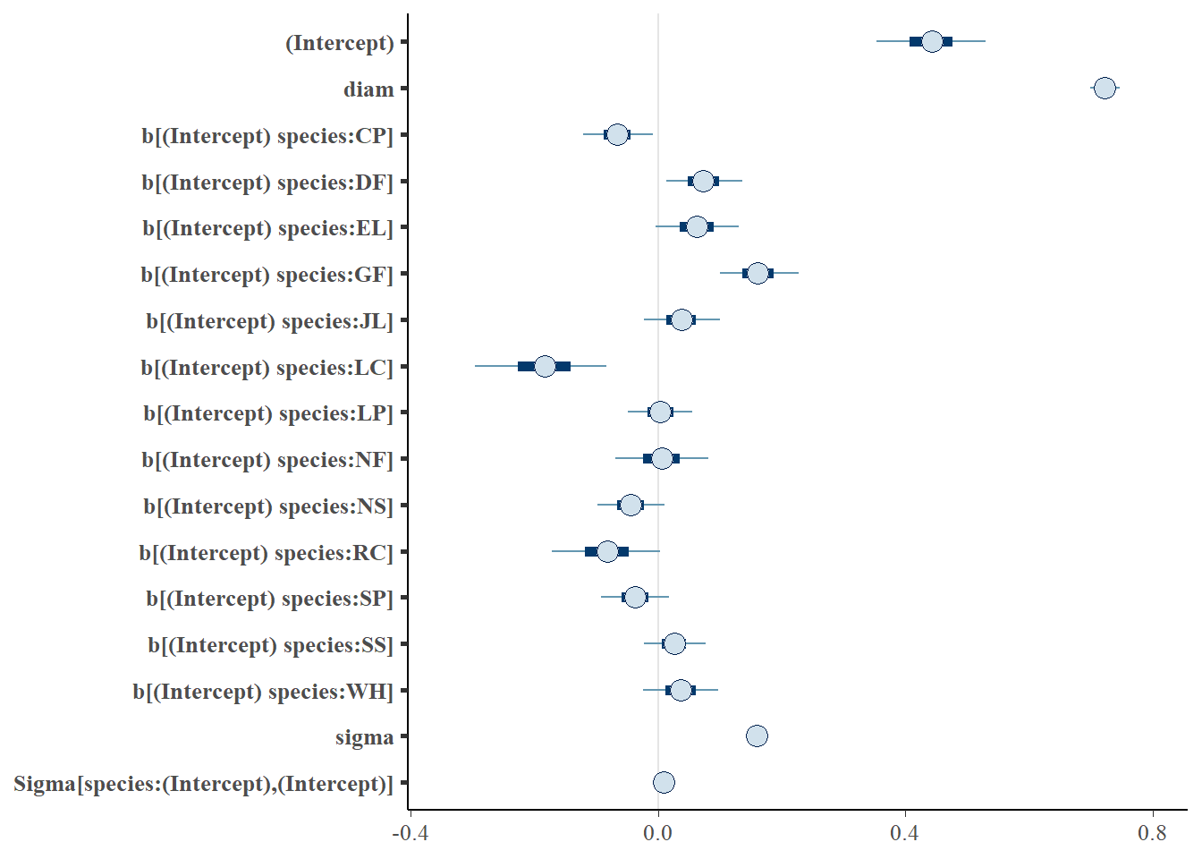
print(m1_stan) # for further information on interpretation: ?print.stanreg
stan_glmer
 family:       gaussian [identity]
 formula:      height ~ diam + (1 | species)
 observations: 1901
------
            Median MAD_SD
(Intercept) 0.4    0.1
diam        0.7    0.0

Auxiliary parameter(s):
      Median MAD_SD
sigma 0.2    0.0

Error terms:
 Groups   Name        Std.Dev.
 species  (Intercept) 0.10
 Residual             0.16
Num. levels: species 13

------
* For help interpreting the printed output see ?print.stanreg
* For info on the priors used see ?prior_summary.stanreg
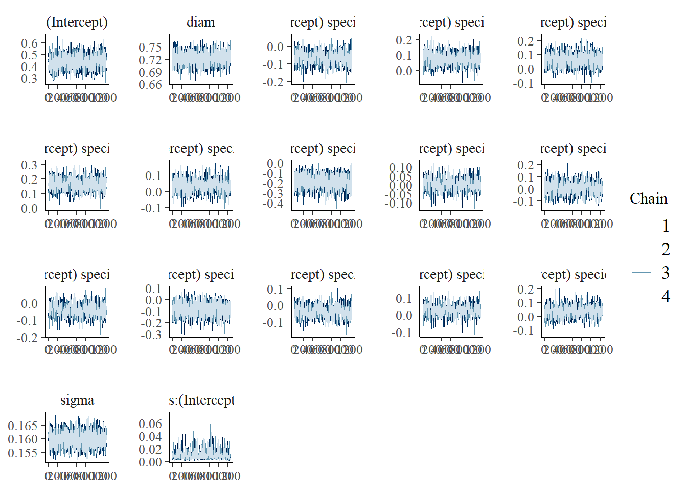
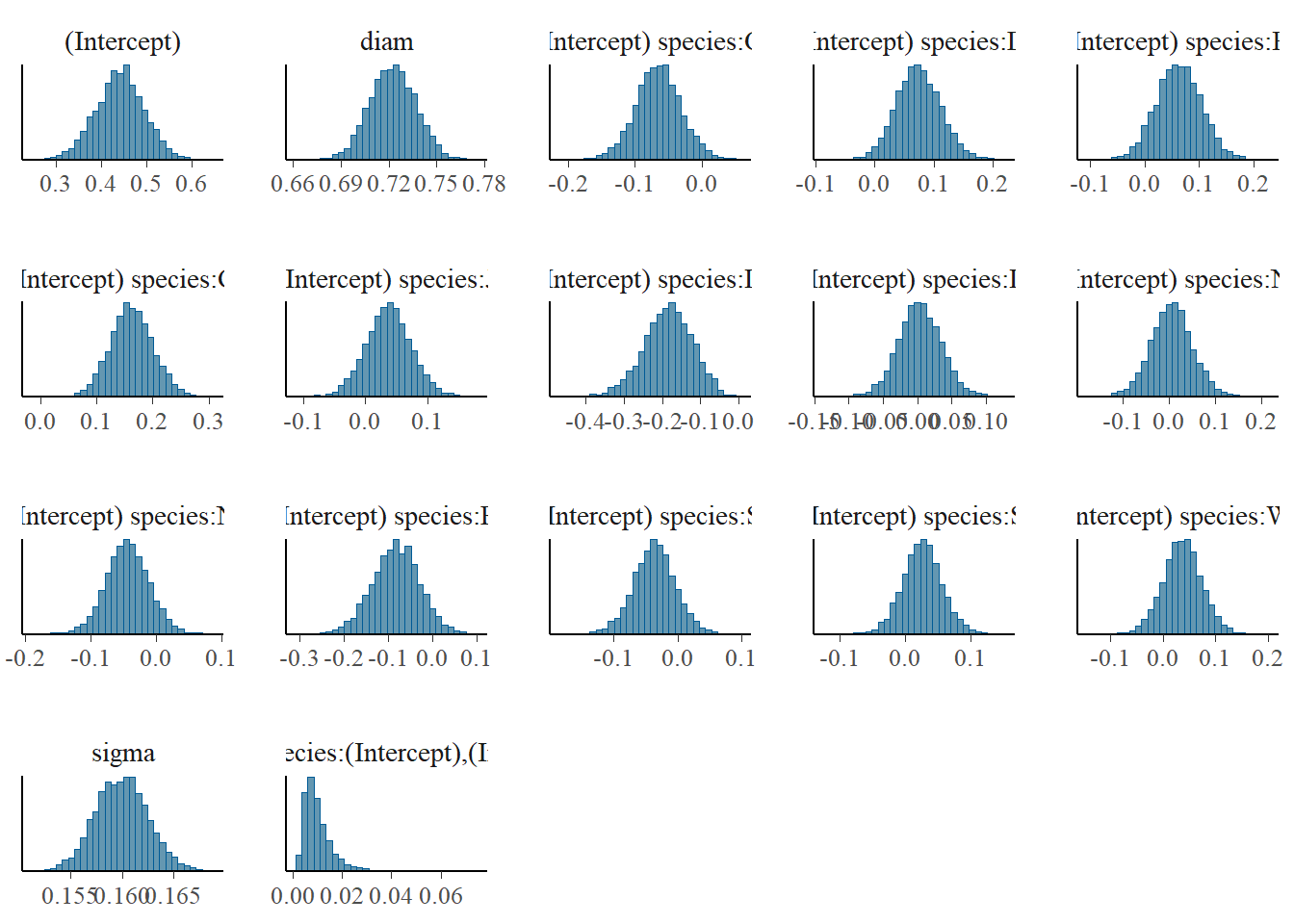
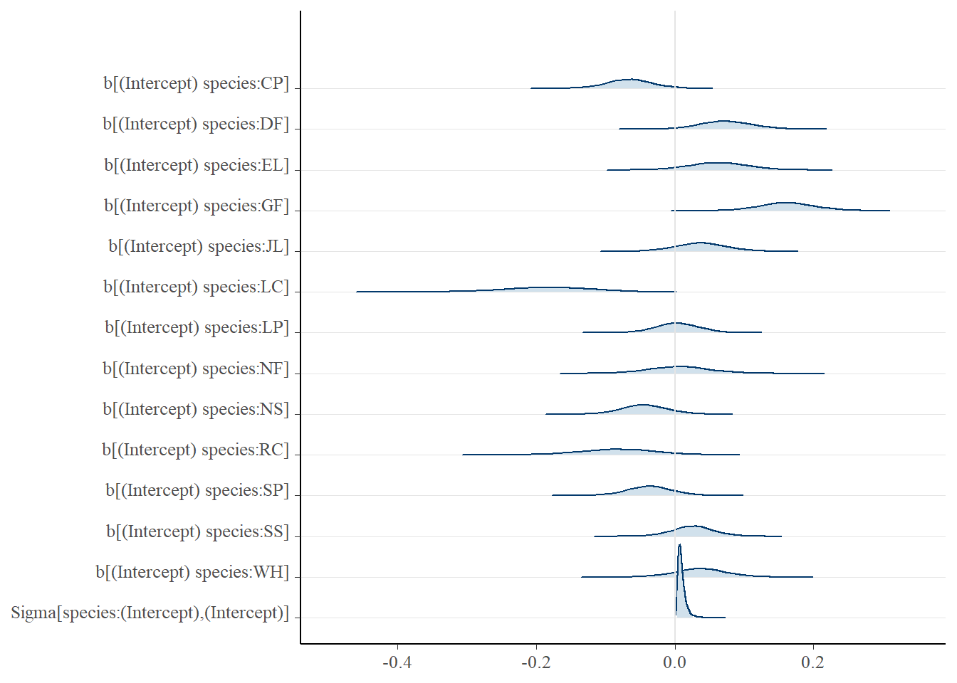
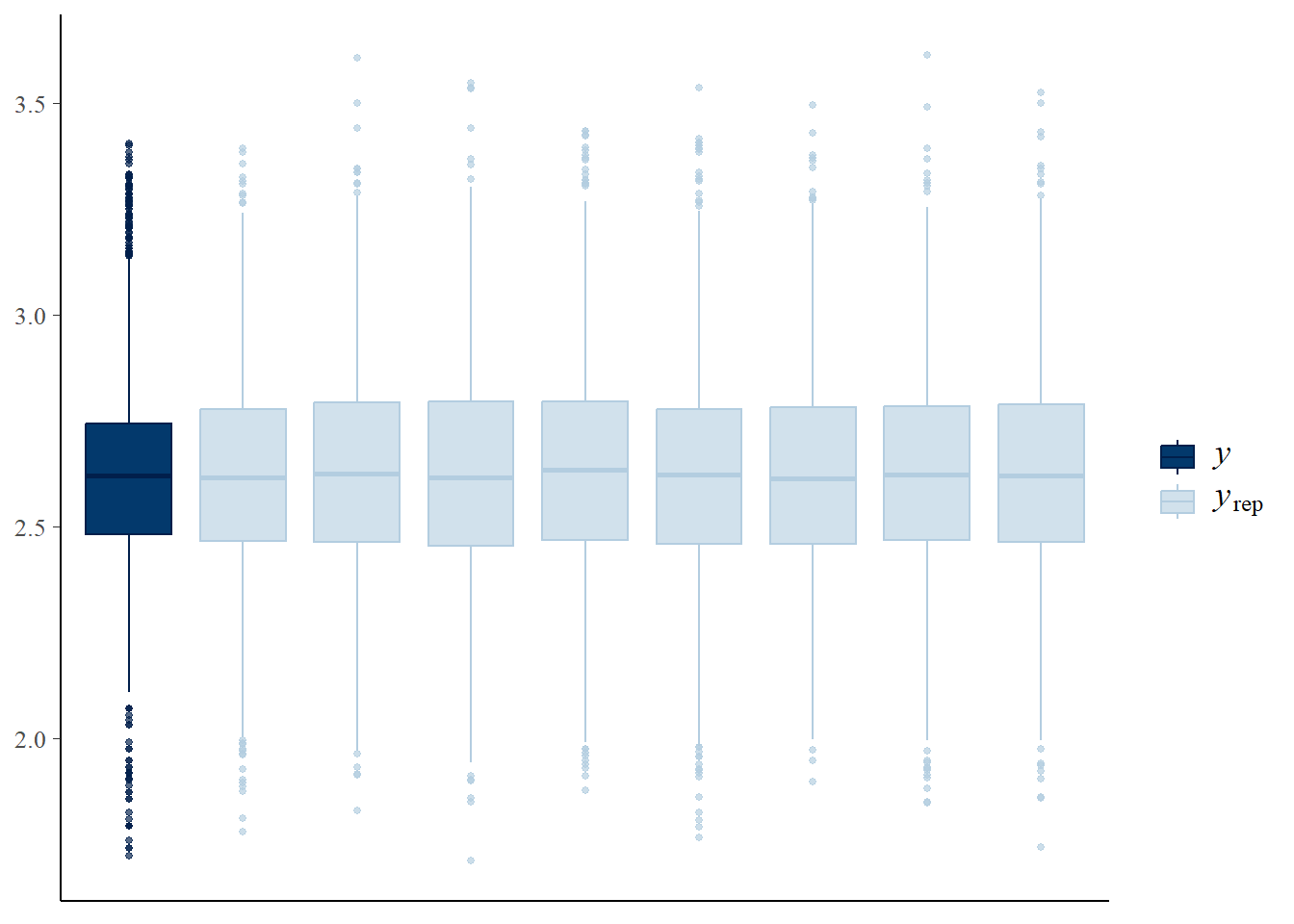
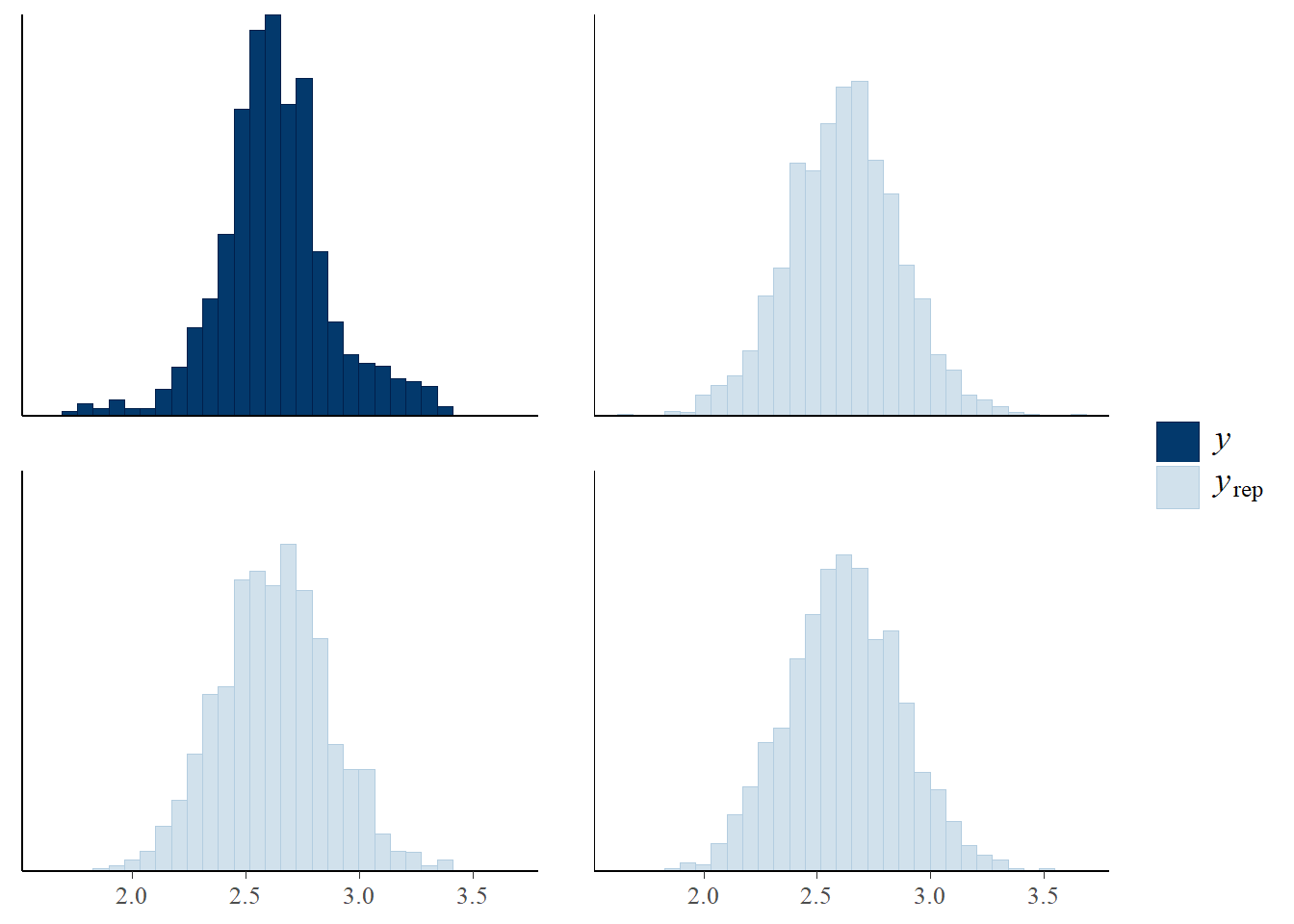
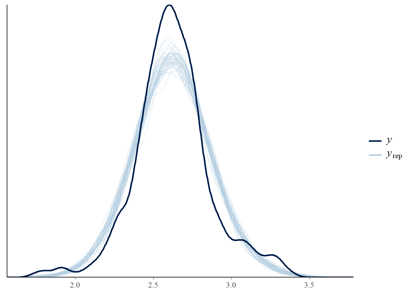
Now let’s take a look at how our modelling process has performed - are our chains behaving, and is their any odd behaviour in our histograms of the MCMC samples? Notice we have a plot for every parameter and grouping level.
`stat_bin()` using `bins = 30`. Pick better value with `binwidth`.
pp_check(m1_stan)
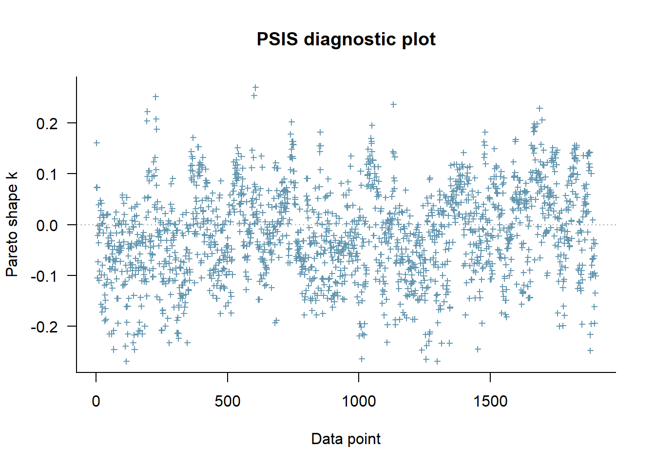
Now let’s apply the leave one out cross-validation using the loo package - are there any problematic influential points?:
library(loo)
Warning: package 'loo' was built under R version 4.4.3
This is loo version 2.8.0
- Online documentation and vignettes at mc-stan.org/loo
- As of v2.0.0 loo defaults to 1 core but we recommend using as many as possible. Use the 'cores' argument or set options(mc.cores = NUM_CORES) for an entire session.
- Windows 10 users: loo may be very slow if 'mc.cores' is set in your .Rprofile file (see https://github.com/stan-dev/loo/issues/94).