library(BayesianTools)
# Create input data for the model
# see help for the VSEM model
PAR <- VSEMcreatePAR(1:2048)

set.seed(123)

# load reference parameter definition (upper, lower prior)
refPars <- VSEMgetDefaults()
# this adds one additional parameter for the likelihood standard deviation (see below)
refPars[12,] <- c(0.1, 0.01, 0.7)
rownames(refPars)[12] <- "error-sd"

# create some simulated test data
# generally recommended to start with simulated data before moving to real data
referenceData <- VSEM(refPars$best[1:11], PAR) # model predictions with reference parameters
referenceData[,1] = 1000 * referenceData[,1]
# this adds the error - needs to conform to the error definition in the likelihood

aobs = referenceData
aobs[,1] = abs(referenceData[,1]) # NEE switches sign so take the absolute value
maobs = colMeans(aobs)

obs = referenceData
obs[,1] <- referenceData[,1] + rnorm(length(referenceData[,1]), sd = maobs[1]*refPars$best[12])
obs[,2] <- referenceData[,2] + rnorm(length(referenceData[,1]), sd = maobs[2]*refPars$best[12])
obs[,3] <- referenceData[,3] + rnorm(length(referenceData[,1]), sd = maobs[3]*refPars$best[12])
obs[,4] <- referenceData[,4] + rnorm(length(referenceData[,1]), sd = maobs[4]*refPars$best[12])

# choose which parmaters to include in the inference
parSel = c(1,3,5,6,9,10,12)Process-based models - Practical
Introduction
In this practical we have an opportunity to put into practise what we learned in the talk by estimating the model parameters of VSEM using the R package “BayesianTools”.
The learning outcomes from the five inferences in this practical are:
- To give practical experience in the Bayesian inference of a process-based model using a Bayesian MCMC approach.
- Show how model structural errors and systematic observational biases can influence Bayesian inference.
- We often have many more observations available for some parts of the ecosytem than for others. Show what issues if any this imbalance can pose to Bayesian inference?
- To give an example of how we should approach the issue of model/observational data errors in Bayesian inference of process-based models?
Work through each section by reading the text and copying and pasting the R code into an R console session. Compare the results that you get with the results presented here and think about any questions asked. We will have a group discussion about the results of each inference and consider any questions asked in the text.
As demonstrated in the talk we first need to load in the BayesianTools package, create the PAR input data and the virtual observations that will be used in the inference.
Bayesian inference of a perfect model
We start by repeating the inference that was demonstrated in the talk. This provides a first opportunity to estimate a process-based model, check that BayesianTools is working correctly and to set a ‘baseline’ against which subsequent inferences can be compared.
First, we define the log likelihood and the prior functions as well as setting the precise MCMC algorithm and the chainlength that we will use. These are essentially the same as the worked example in the talk. We then run the inference using the runMCMC function.
likelihood <- function(par, sum = TRUE){
# set parameters that are not inferred to default values
x = refPars$best
x[parSel] = par
predicted <- VSEM(x[1:11], PAR) # replace here VSEM with your model
predicted[,1] = 1000 * predicted[,1] # this is just rescaling
diff <- c(predicted[,1] - obs[,1])
llValues1 <- dnorm(diff, sd = x[12]*maobs[1], log = T)
diff <- c(predicted[,2] - obs[,2])
llValues2 <- dnorm(diff, sd = x[12]*maobs[2], log = T)
diff <- c(predicted[,3] - obs[,3])
llValues3 <- dnorm(diff, sd = x[12]*maobs[3], log = T)
# univariate normal likelihood. Note that there is a parameter involved here that is fit
return(sum(llValues1,llValues2,llValues3))
}
prior <- createUniformPrior(lower = refPars$lower[parSel],
upper = refPars$upper[parSel], best = refPars$best[parSel])
bayesianSetup <- createBayesianSetup(likelihood, prior, names = rownames(refPars)[parSel])
settings <- list(iterations = 60000, nrChains = 2)
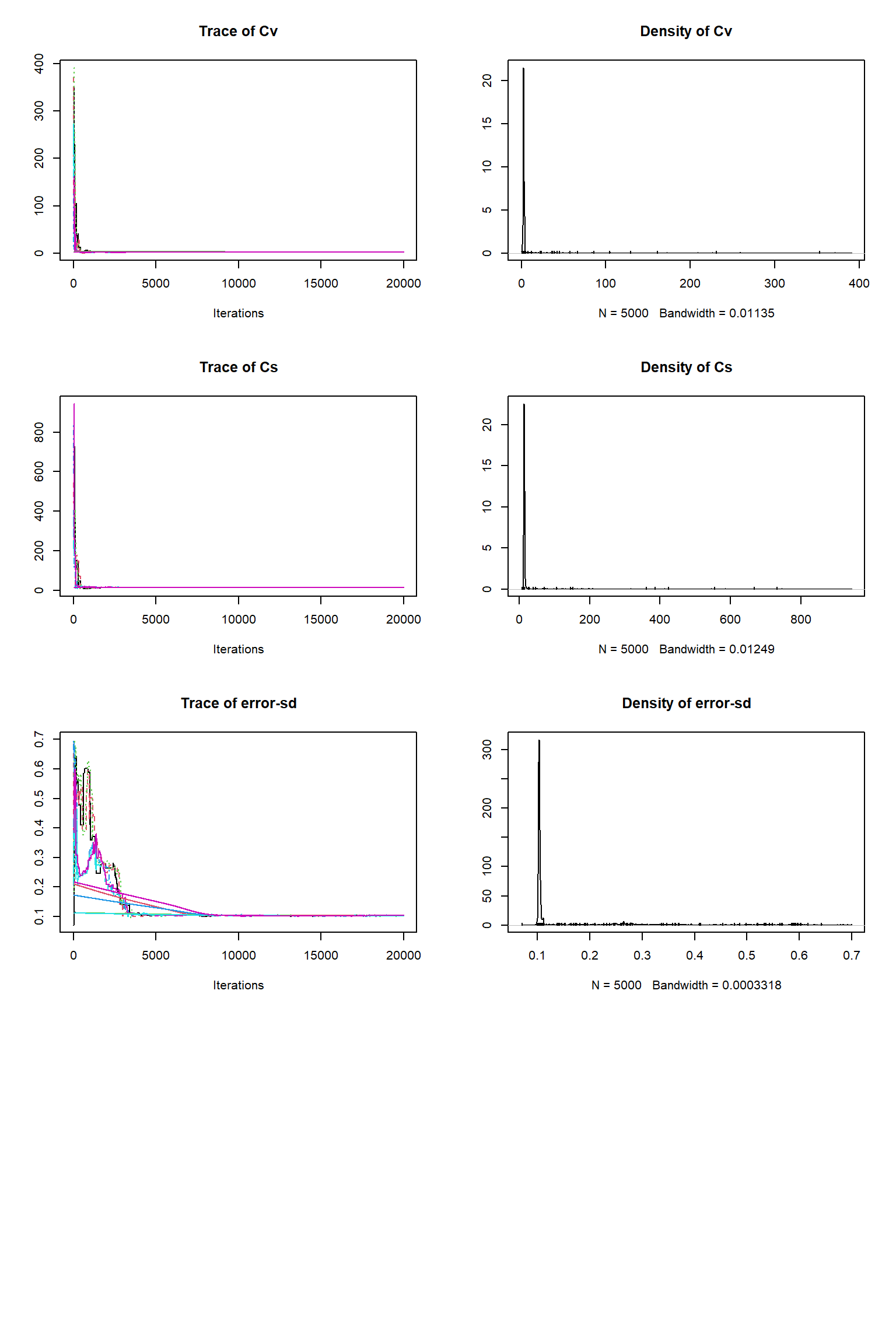
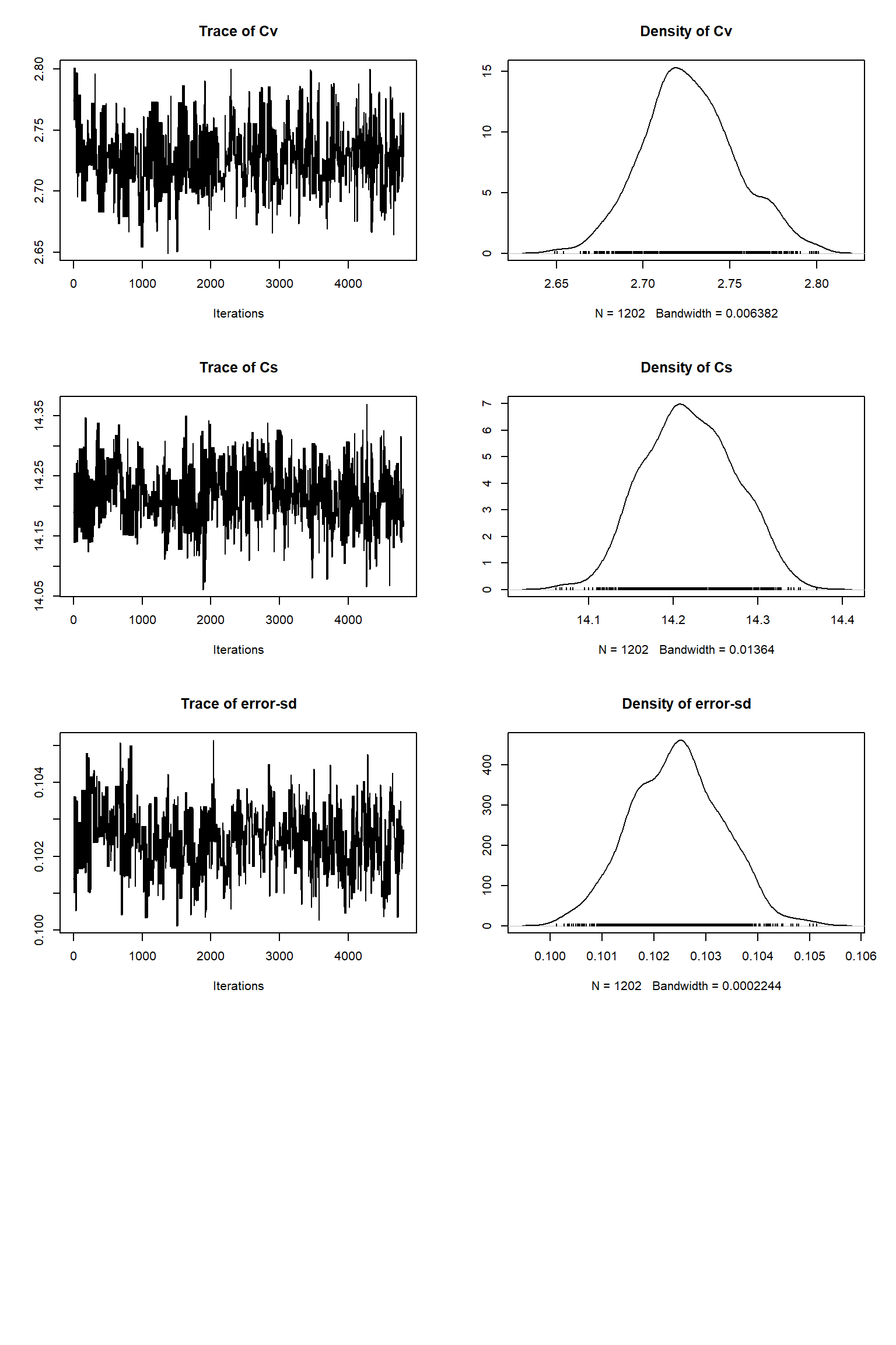
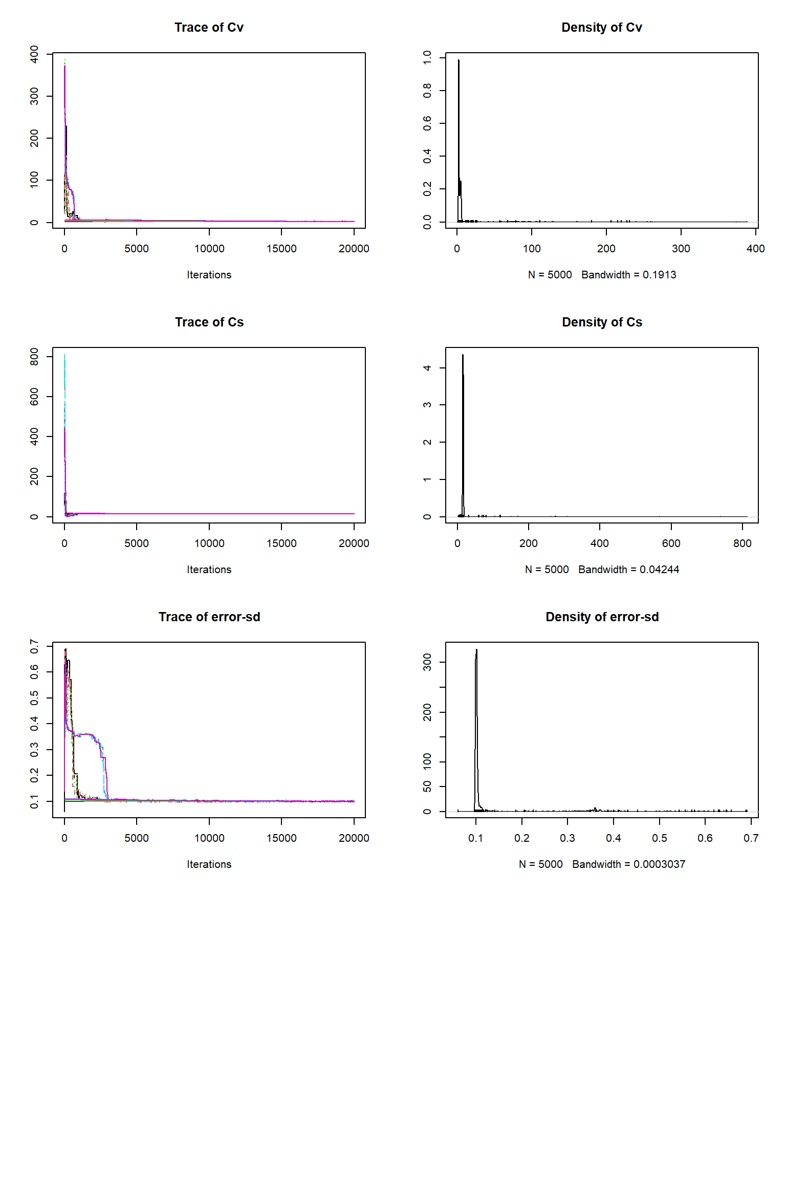
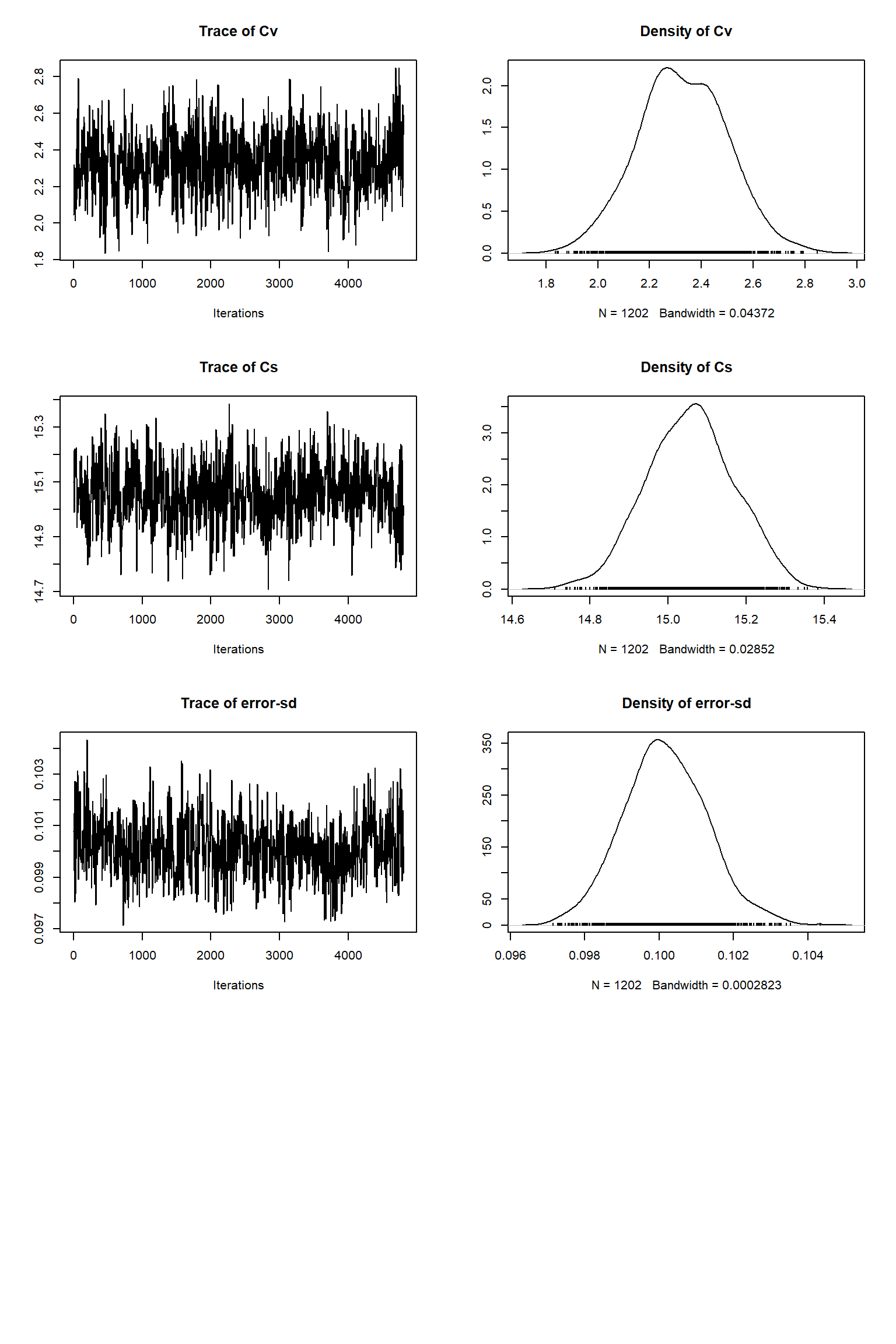
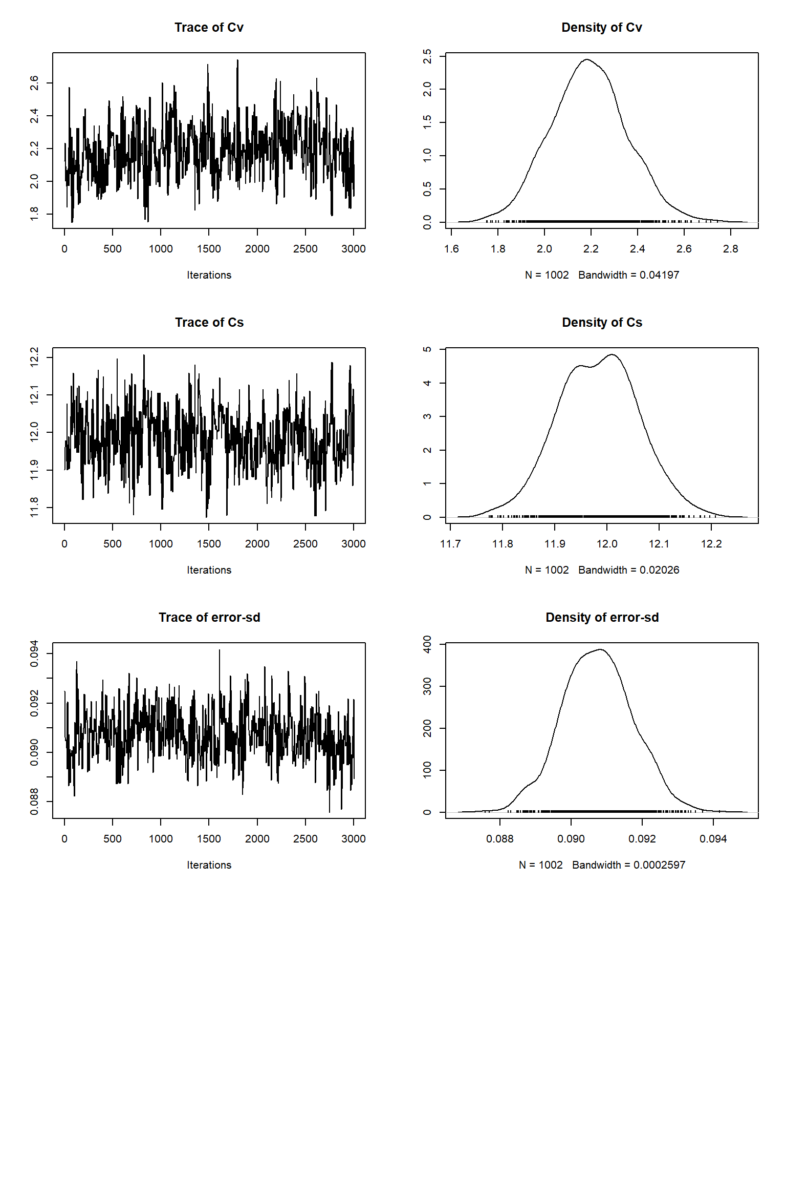
out <- runMCMC(bayesianSetup = bayesianSetup, sampler = "DEzs", settings = settings)As in the talk, we plot the MCMC chain to check for convergence. We also remove the burn-in, resample the MCMC chain and rerun VSEM with the sample and plot model predictions with the posterior uncertainty.
tracePlot(sampler = out)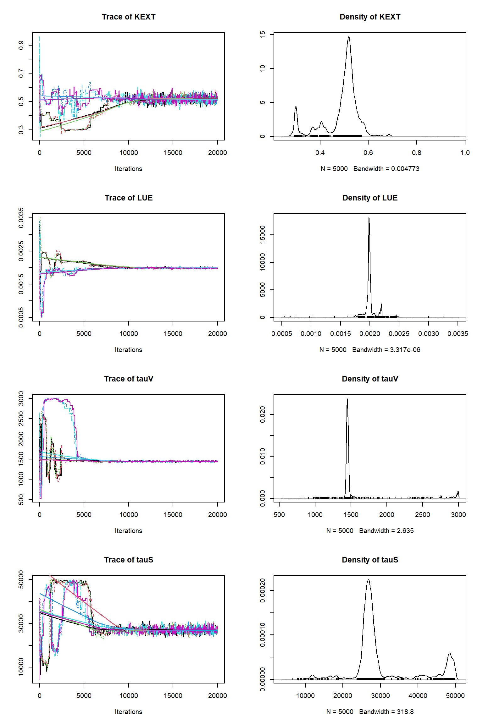
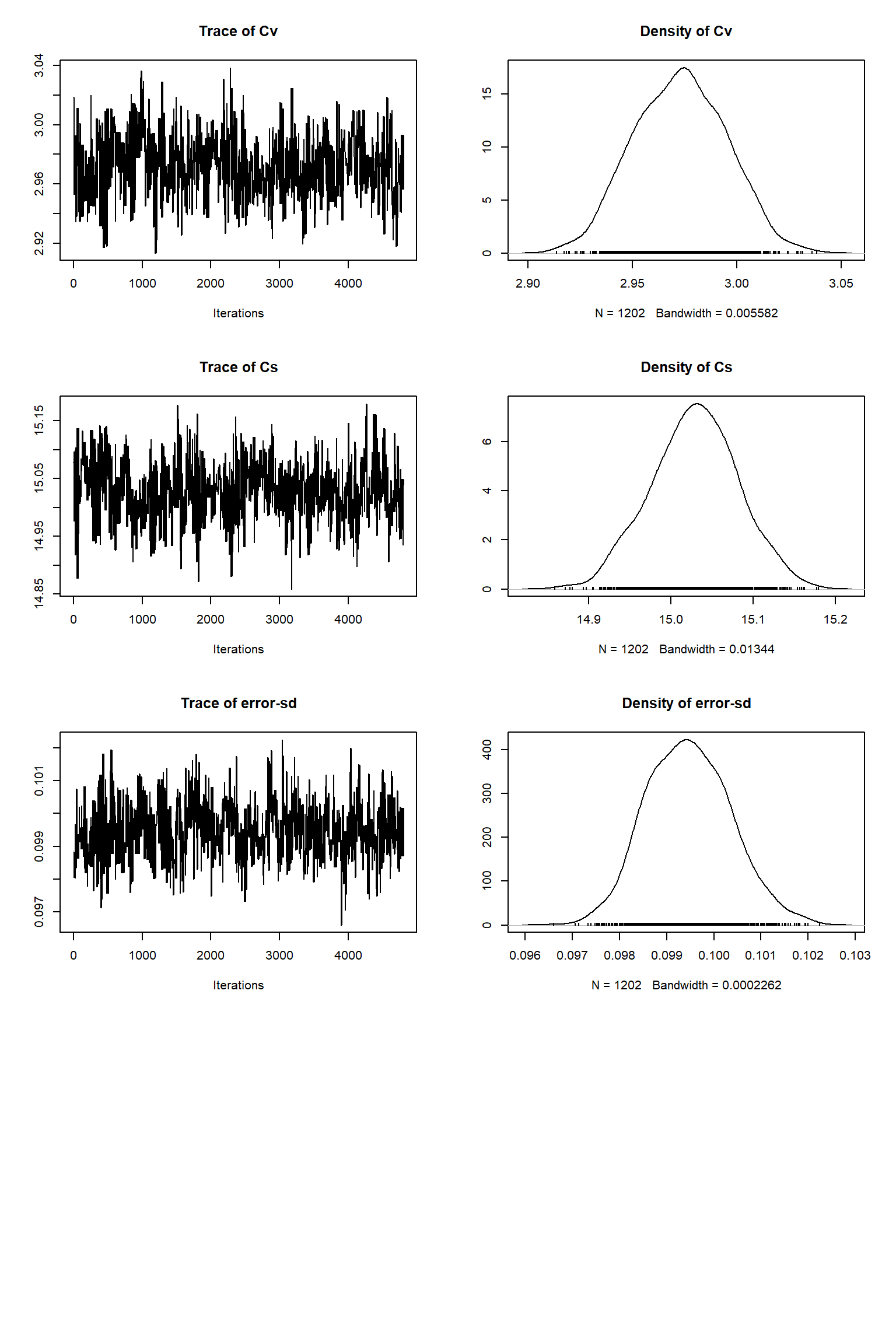
bout = getSample(out,thin=10,start=12000)
tracePlot(sampler = bout)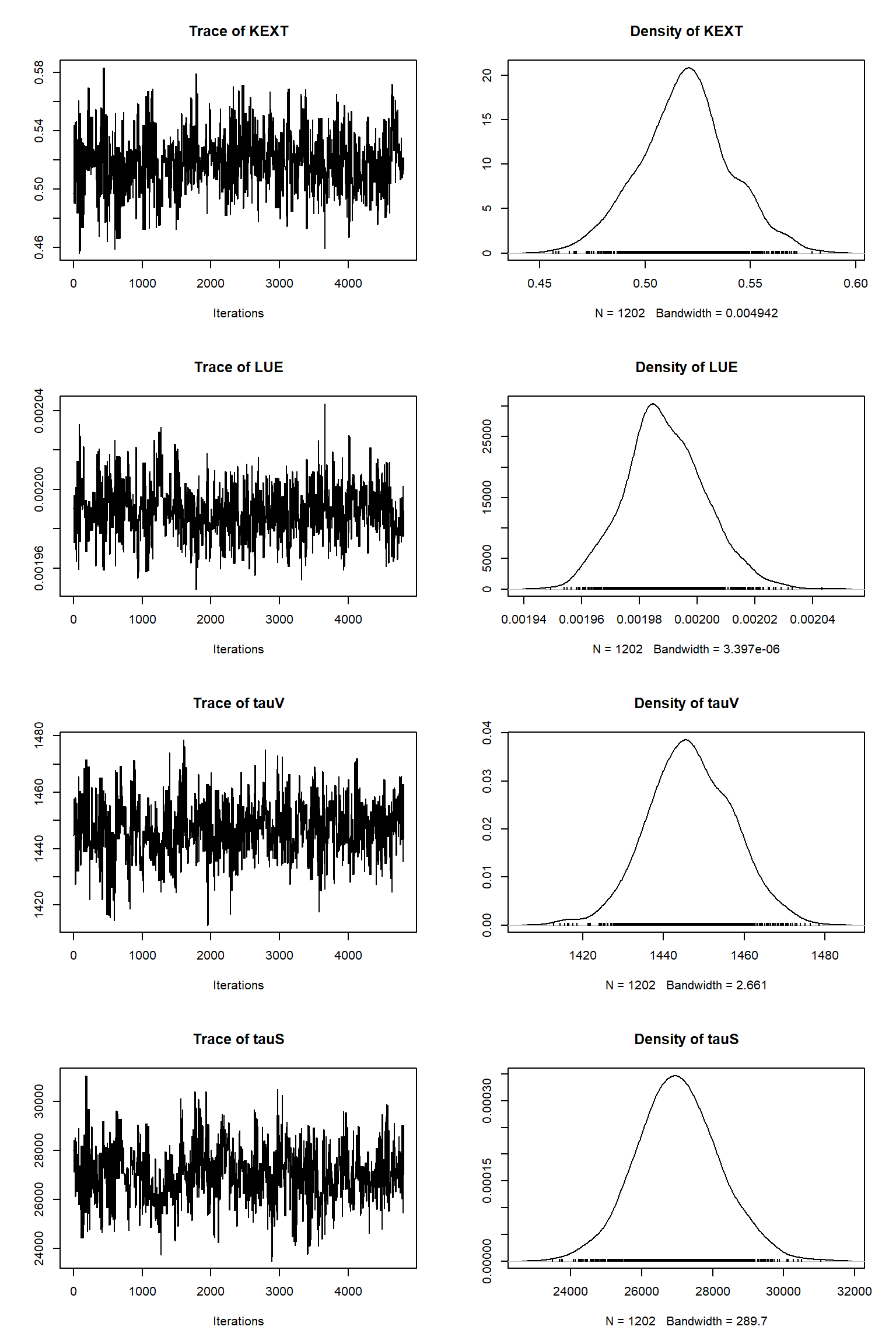
createPredictions <- function(par){
  # set the parameters that are not inferred to default values
  x = refPars$best
  x[parSel] = par
  predicted <- VSEM(x[1:11], PAR) # replace here VSEM with your model
  predicted[,1] = predicted[,1] * 1000
  return(predicted[,ifld])
}
# Create an error function
createError <- function(mean, par){
  return(rnorm(length(mean), mean = mean, sd = par[7]*maobs[ifld]))
}

ifld<-2
myObs<-obs[,ifld]
plotTimeSeriesResults(sampler = bout, model = createPredictions, observed = myObs,
                      plotResiduals=FALSE, error = createError, prior = FALSE, main = "Cv posterior predictive")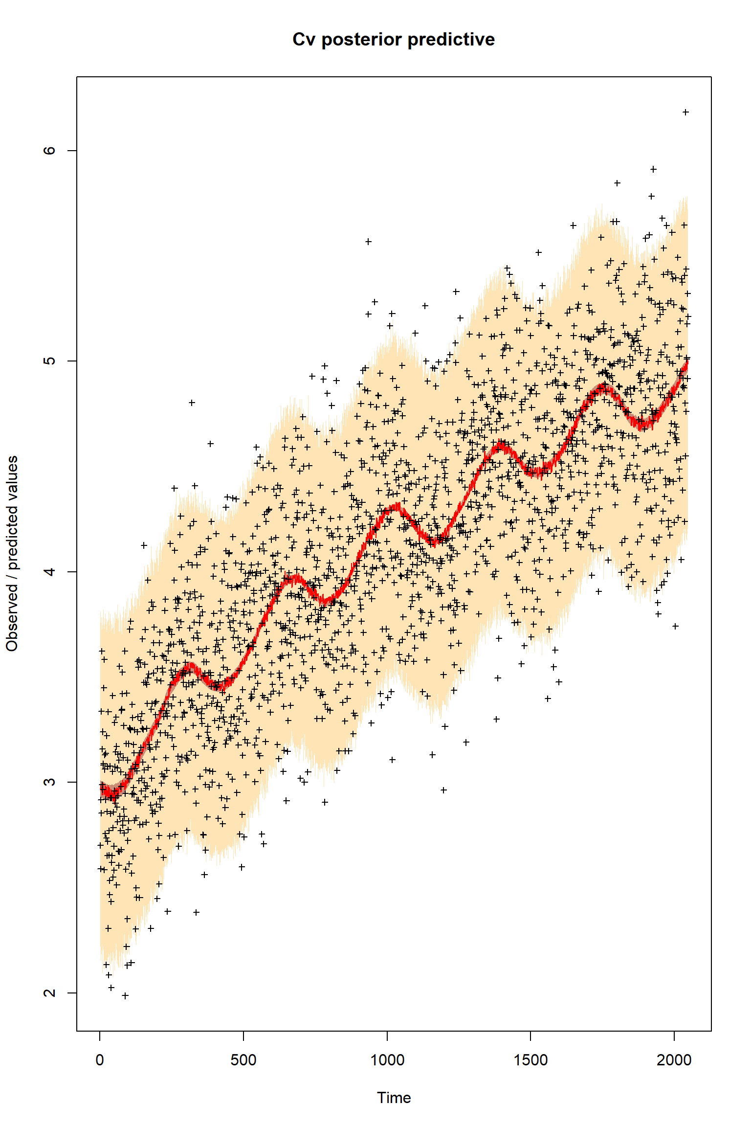
ifld<-3
myObs<-obs[,ifld]
plotTimeSeriesResults(sampler = bout, model = createPredictions, observed = myObs,
                      plotResiduals=FALSE, error = createError, prior = FALSE, main = "Cs posterior predictive")
Looking at the plots, everything so far is unsurprisingly similar to what we had in the talk. If you get similar results to these then the BayesianTools package is working as expected on your machine.
Before going on to make other inferences we discuss the assumptions implied in the uncertainty model.
The uncertainty model
The choices that we have made in the prior and likelihood functions express the uncertainty model that we have for the model parameters and the observations.
We know that the prior uncertainty expresses our uncertainty about the model parameters before the inference. The prior uncertainty function that we have used so far makes the assumption that the parameter uncertainties are independent. This is a common assumption to make for process-based models as covariances between parameters are often complex and so are unlikely to be well known initially.
In the likelihood, we express the uncertainty in the observations given that the parameters are correct. In using the Gaussian likelihood function “dnorm”, we have also made the assumption that uncertainty in the observations are independent. This was a good assumption in our case as we created the virtual observations from the model outputs by adding noise from a Gaussian distribution without covariances.
As expressed in the function above we form the log likelihood by differencing the model and the observations. So what we are actually assuming is that model/observational differences are independent. In our case this is again a good assumption as the only difference between the model and data is the Gaussian noise that we added. Since both the prior uncertainty and the observational random noise are represented in the inference we can be confident that the inference represents all the uncertainties.
As discussed in the talk, unfortunately, real world PBMs are never perfect representations of the ecosystem and observations will also often have systematic biases and representative errors. In addition, since these errors are often unknown it can be very challenging to correct them through model development and correcting biases, this also affects our ability to adequately represent the uncertainty of model structural errors and observational biases in the inference. The presence of these errors means that model - data differences are never independent - yet this is a common assumption made in the uncertainty model expressed in the likelihoods used in the Bayesian inference of PBMs.
Questions
Would you say that our prior choice here is informative or uninformative?
What is the likely relationship between the posterior and the likelihood in this inference?
In the following inference we will introduce a known error into the VSEM model so that we can analyse the impact that this can have on a inference.
Bayesian inference of a model with a structural error
We introduce the model structural error in the likelihood function below by setting the Av parameter to 1 so that all the NPP is allocated to the vegetation carbon pool and none to the root pool. We also initialise the root carbon pool to zero. Thus in effect, we have removed the root carbon process from the model. Unknown and hence missing model processes are a common form of model structural error. The inference is otherwise the same as before.
likelihood <- function(par, sum = TRUE){
  # set parameters that are not inferred to default values
  x = refPars$best
  x[8]=1.0
  x[11]=0.0
  x[parSel] = par
  predicted <- VSEM(x[1:11], PAR) # replace here VSEM with your model
  predicted[,1] = 1000 * predicted[,1] # this is just rescaling
  diff       <- c(predicted[,1] - obs[,1])
  llValues1  <- dnorm(diff, sd = x[12]*maobs[1], log = T)
  diff       <- c(predicted[,2] - obs[,2])
  llValues2  <- dnorm(diff, sd = x[12]*maobs[2], log = T)
  diff       <- c(predicted[,3] - obs[,3])
  llValues3  <- dnorm(diff, sd = x[12]*maobs[3], log = T)
  # univariate normal likelihood. Note that there is a parameter involved here that is fit
  return(sum(llValues1,llValues2,llValues3))
}

bayesianSetup <- createBayesianSetup(likelihood, prior, names = rownames(refPars)[parSel])

settings <- list(iterations = 60000, nrChains = 2)

out <- runMCMC(bayesianSetup = bayesianSetup, sampler = "DEzs", settings = settings)tracePlot(sampler = out)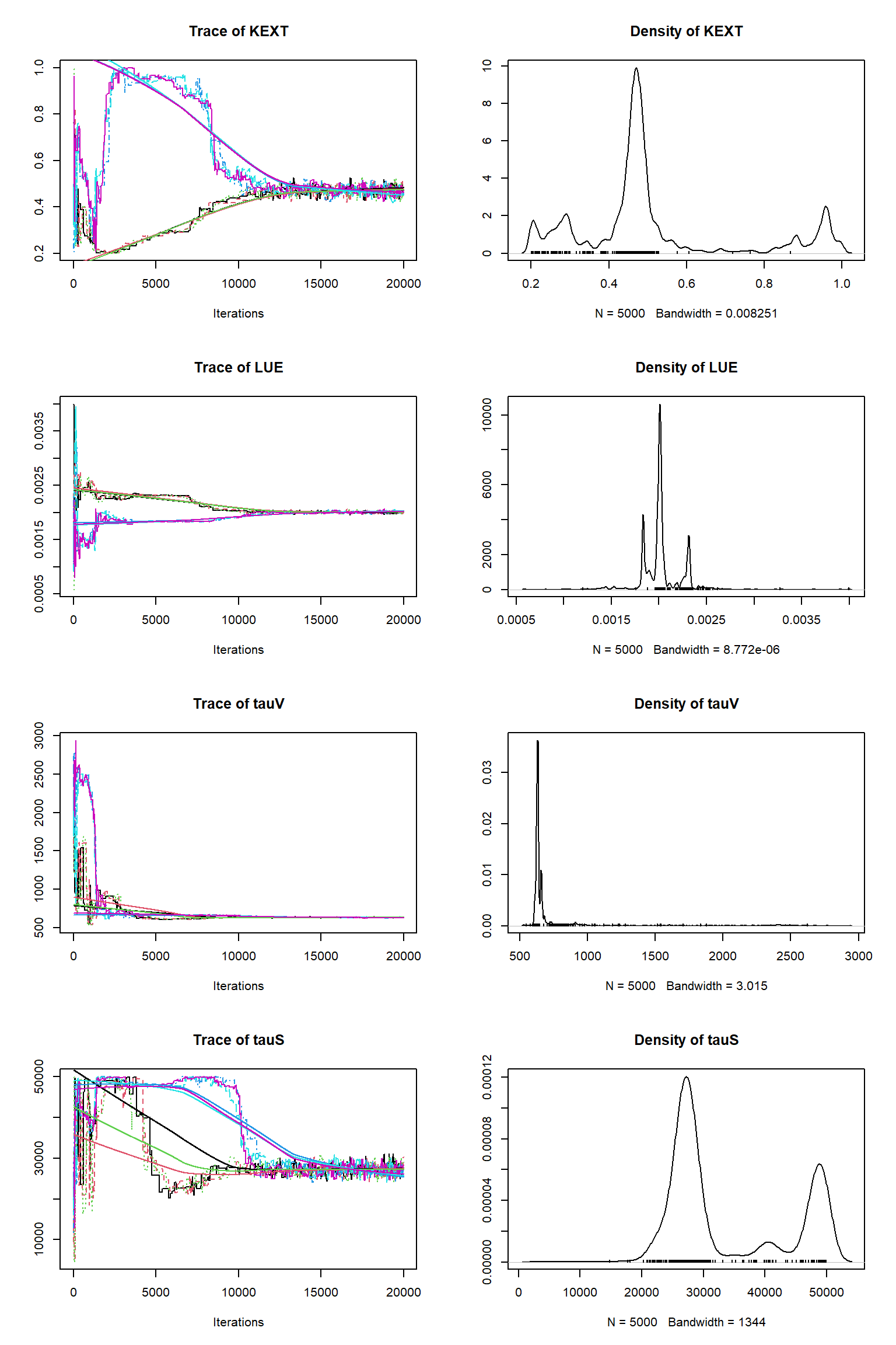
bout = getSample(out,thin=10,start=12000)
tracePlot(sampler = bout)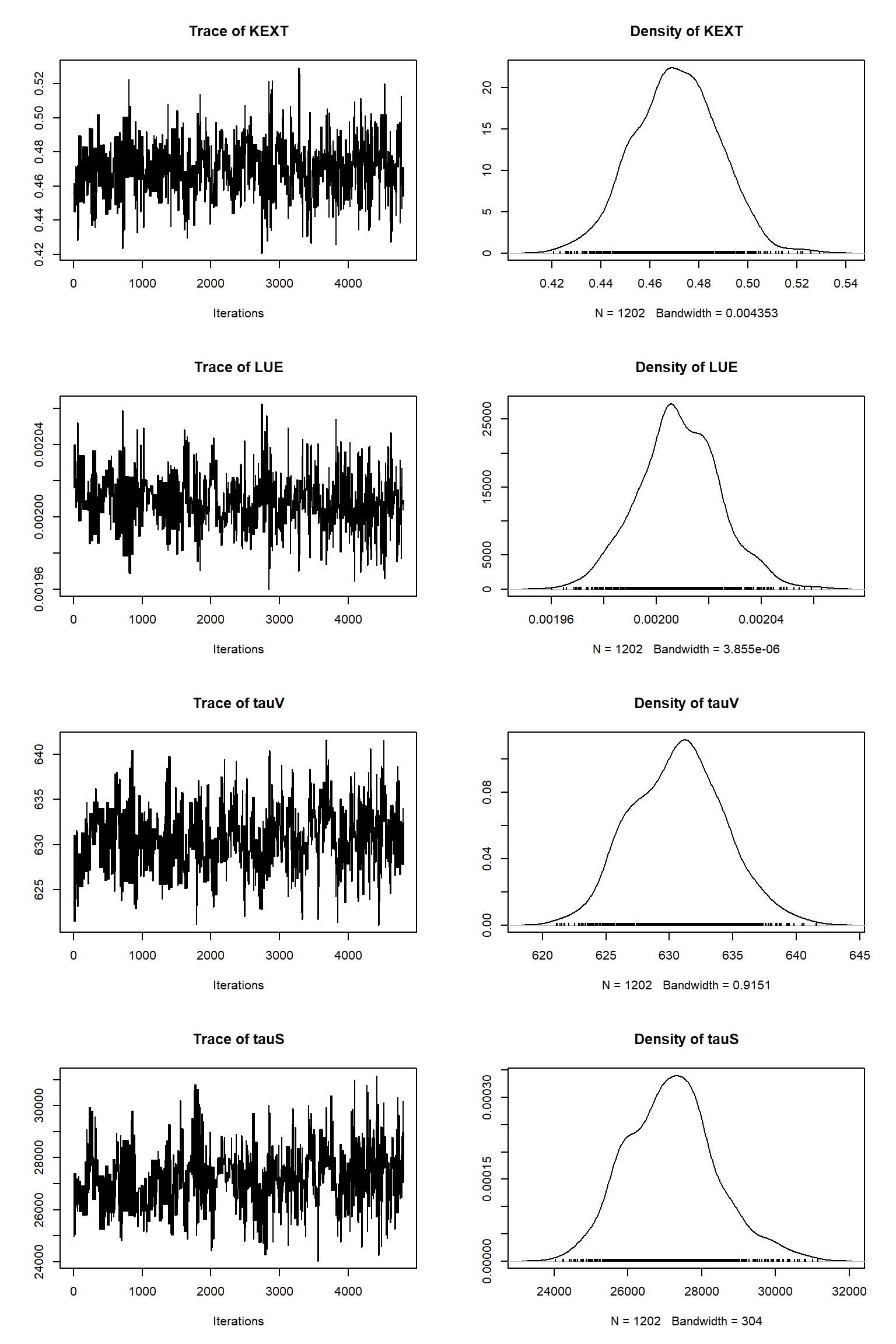
createPredictionsErr <- function(par){
  # set the parameters that are not inferred to default values
  x = refPars$best
  x[8]=1.0
  x[11]=0.0
  x[parSel] = par
  predicted <- VSEM(x[1:11], PAR) # replace here VSEM with your model
  predicted[,1] = predicted[,1] * 1000
  return(predicted[,ifld])
}

ifld<-2
myObs<-obs[,ifld]
plotTimeSeriesResults(sampler = bout, model = createPredictionsErr, observed = myObs,
                      plotResiduals=FALSE, error = createError, prior = FALSE, main = "Cv posterior predictive")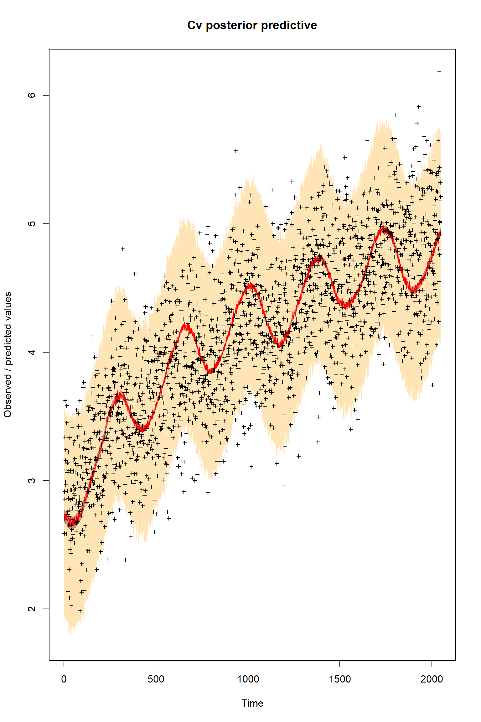
ifld<-3
myObs<-obs[,ifld]
plotTimeSeriesResults(sampler = bout, model = createPredictionsErr, observed = myObs,
                      plotResiduals=FALSE, error = createError, prior = FALSE, main = "Cs posterior predictive")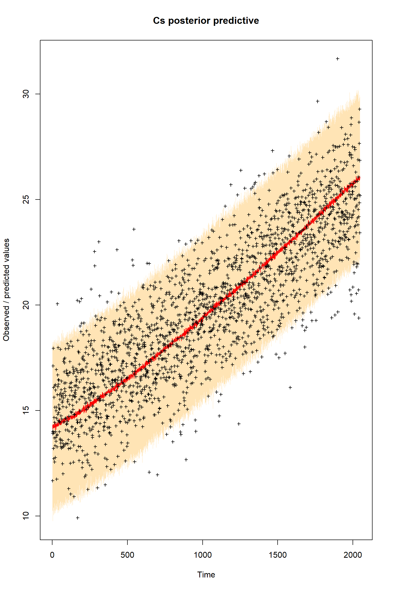
Given that this is a significant model error it is quite striking how well the model fits the observations after the inference. It is almost as if the the error was not present at all.
Questions
Is this what you were expecting?
What do you think has happended here so that the model apparently seems to perform well even with this significant error present?
Large imbalances in available observational data
Measuring some parts of the ecosytem is often far more labourious than others; for example soil measurements. Hence it is common to have a large imbalance in the number of observations available for some parts of the system than others. We simulate this here by removing the bulk of the observations from the vegetative carbon pool, giving us a two orders of magnitude imbalance in the observations. This size of imbalance is common in Bayesian inference of ecosystem PBMs. This in addition to the presence of model errors is getting closer to the kind of inference that you are likely to find in a ‘real world’ situation.
obsSel=seq(2,2048,400)
likelihood <- function(par, sum = TRUE){
  # set parameters that are not inferred to default values
  x = refPars$best
  x[8]=1.0
  x[11]=0.0
  x[parSel] = par
  predicted <- VSEM(x[1:11], PAR) # replace here VSEM with your model
  predicted[,1] = 1000 * predicted[,1] # this is just rescaling
  diff       <- c(predicted[,1] - obs[,1])
  llValues1  <- dnorm(diff, sd = x[12]*maobs[1], log = T)
  diff       <- c(predicted[obsSel,2] - obs[obsSel,2])
  llValues2  <- dnorm(diff, sd = x[12]*maobs[2], log = T)
  diff       <- c(predicted[,3] - obs[,3])
  llValues3  <- dnorm(diff, sd = x[12]*maobs[3], log = T)

  # univariate normal likelihood. Note that there is a parameter involved here that is fit
  return(sum(llValues1,llValues2,llValues3))
}

bayesianSetup <- createBayesianSetup(likelihood, prior, names = rownames(refPars)[parSel])

settings <- list(iterations = 60000, nrChains = 2)

out <- runMCMC(bayesianSetup = bayesianSetup, sampler = "DEzs", settings = settings)tracePlot(sampler = out)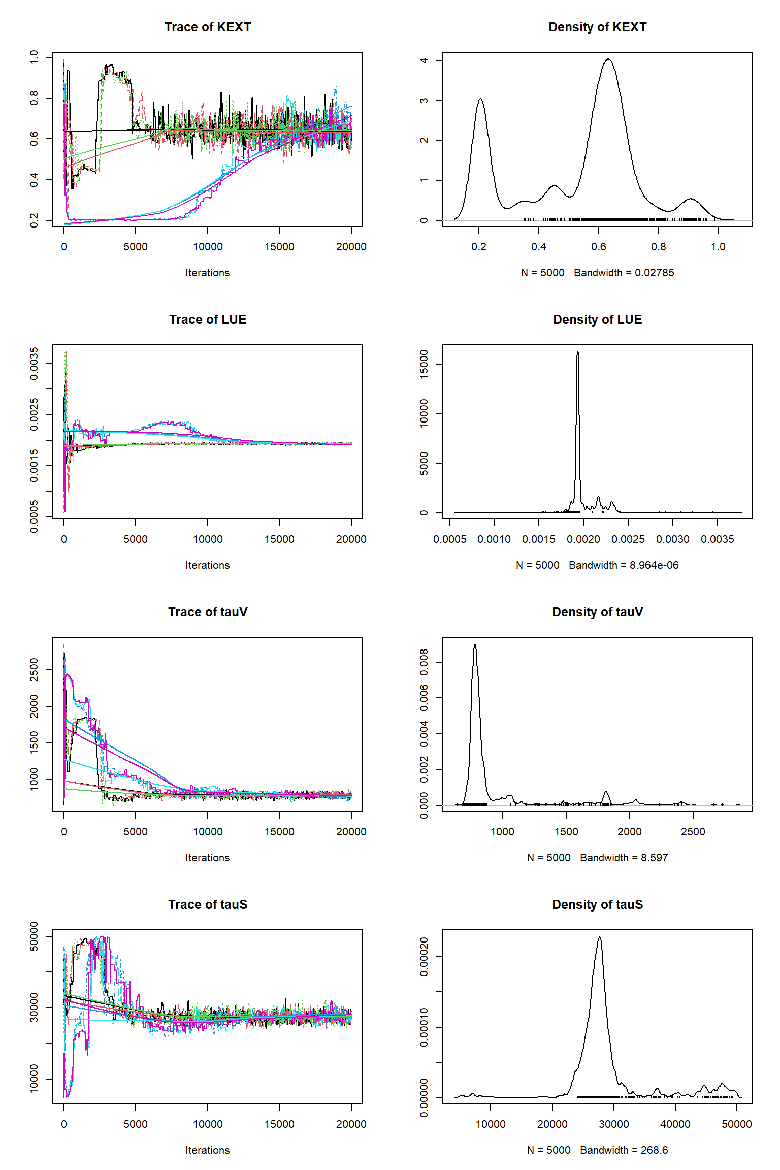
bout = getSample(out,thin=10,start=12000)
tracePlot(sampler = bout)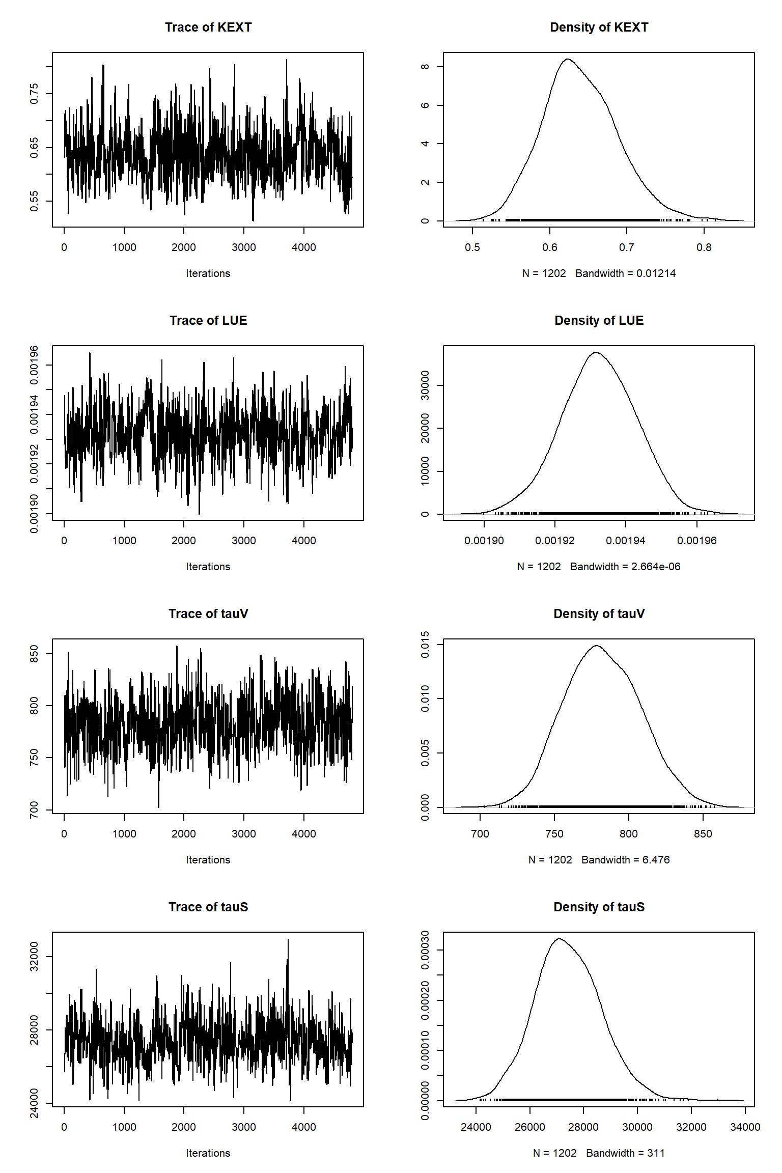
ifld<-2
myObs<-obs[,ifld]
myObs[-obsSel] <- NA
plotTimeSeriesResults(sampler = bout, model = createPredictionsErr, observed = myObs,
                      plotResiduals=FALSE, error = createError, prior = FALSE, main = "Cv posterior predictive")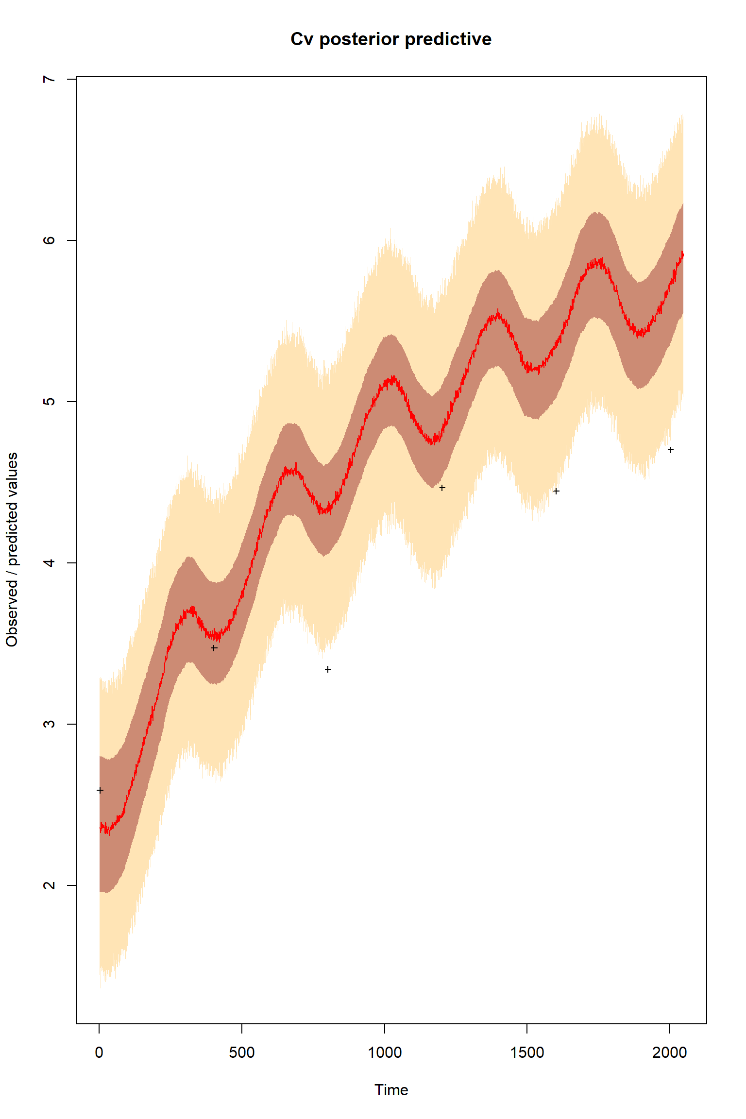
ifld<-3
myObs<-obs[,ifld]
plotTimeSeriesResults(sampler = bout, model = createPredictionsErr, observed = myObs,
                      plotResiduals=FALSE, error = createError, prior = FALSE, main = "Cs posterior predictive")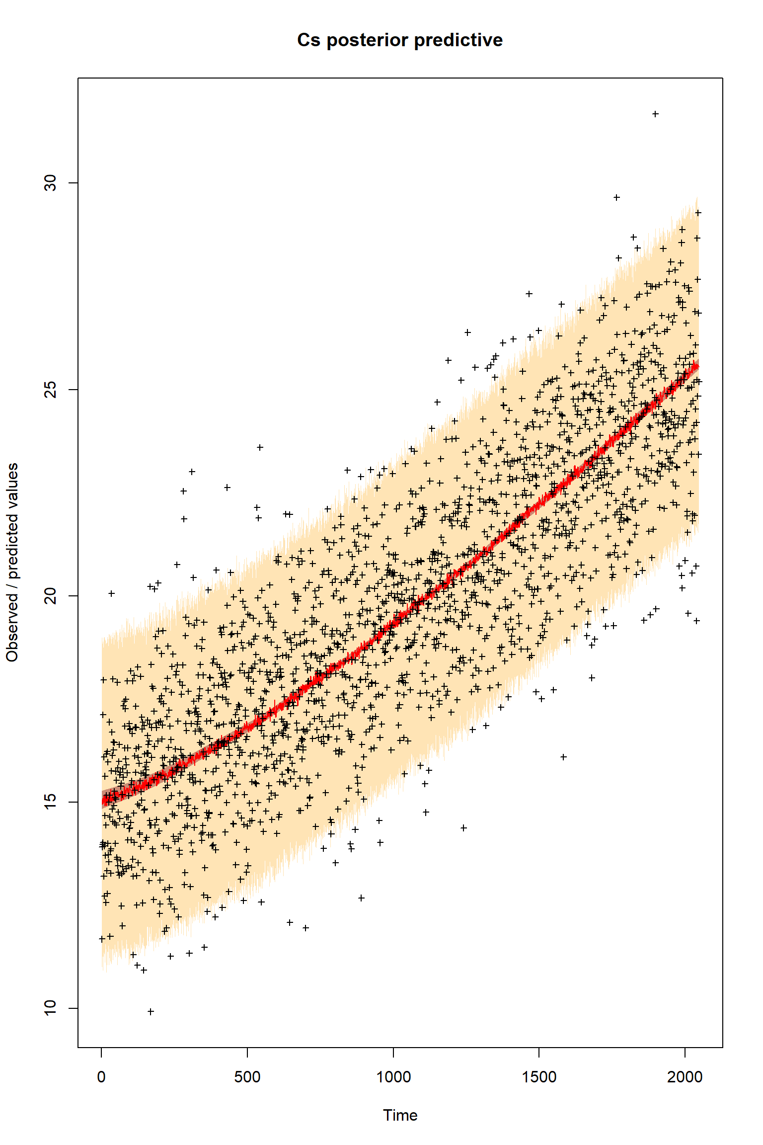
Questions
The inference against the plentiful soil data looks fine but is significantly poorer than against the sparse vegetative carbon data. It looks as though the vegatative carbon data is being somewhat ignored. Why do you think this has happend? Does this suggest that there can be issues with Bayesian inference where there are large imbalences in the numbers of obervations? How might we solve this? A common approach is to thin out the number of plentiful observations to restore balance - what do we think about this?
Systematic biases in observational data
Unfortunately it is not only models that can have large structural errors present. Large systematic biases can also be present in the observations. As discussed in the talk, these can be due to a number of different factors (instrument error, observer error poor representation of the ecosystem being modelled etc).
Here we simulate a systematic bias by multiplying the soil carbon observations by 0.8. To keep things simple, we have removed the model structural error but have retained the large imbalance in the data from before.
eobs <- 0.8*obs[,3]

obsSel=seq(2,2048,400)
likelihood <- function(par, sum = TRUE){
  # set parameters that are not inferred to default values
  x = refPars$best
  x[parSel] = par
  predicted <- VSEM(x[1:11], PAR) # replace here VSEM with your model
  predicted[,1] = 1000 * predicted[,1] # this is just rescaling
  diff       <- c(predicted[,1] - obs[,1])
  llValues1  <- dnorm(diff, sd = x[12]*maobs[1], log = T)
  diff       <- c(predicted[obsSel,2] - obs[obsSel,2])
  llValues2  <- dnorm(diff, sd = x[12]*maobs[2], log = T)
  diff       <- c(predicted[,3] - eobs)
  llValues3  <- dnorm(diff, sd = x[12]*maobs[3], log = T)
  # univariate normal likelihood. Note that there is a parameter involved here that is fit
  return(sum(llValues1,llValues2,llValues3))
}

bayesianSetup <- createBayesianSetup(likelihood, prior, names = rownames(refPars)[parSel])

settings <- list(iterations = 60000, nrChains = 2)

out <- runMCMC(bayesianSetup = bayesianSetup, sampler = "DEzs", settings = settings)tracePlot(sampler = out)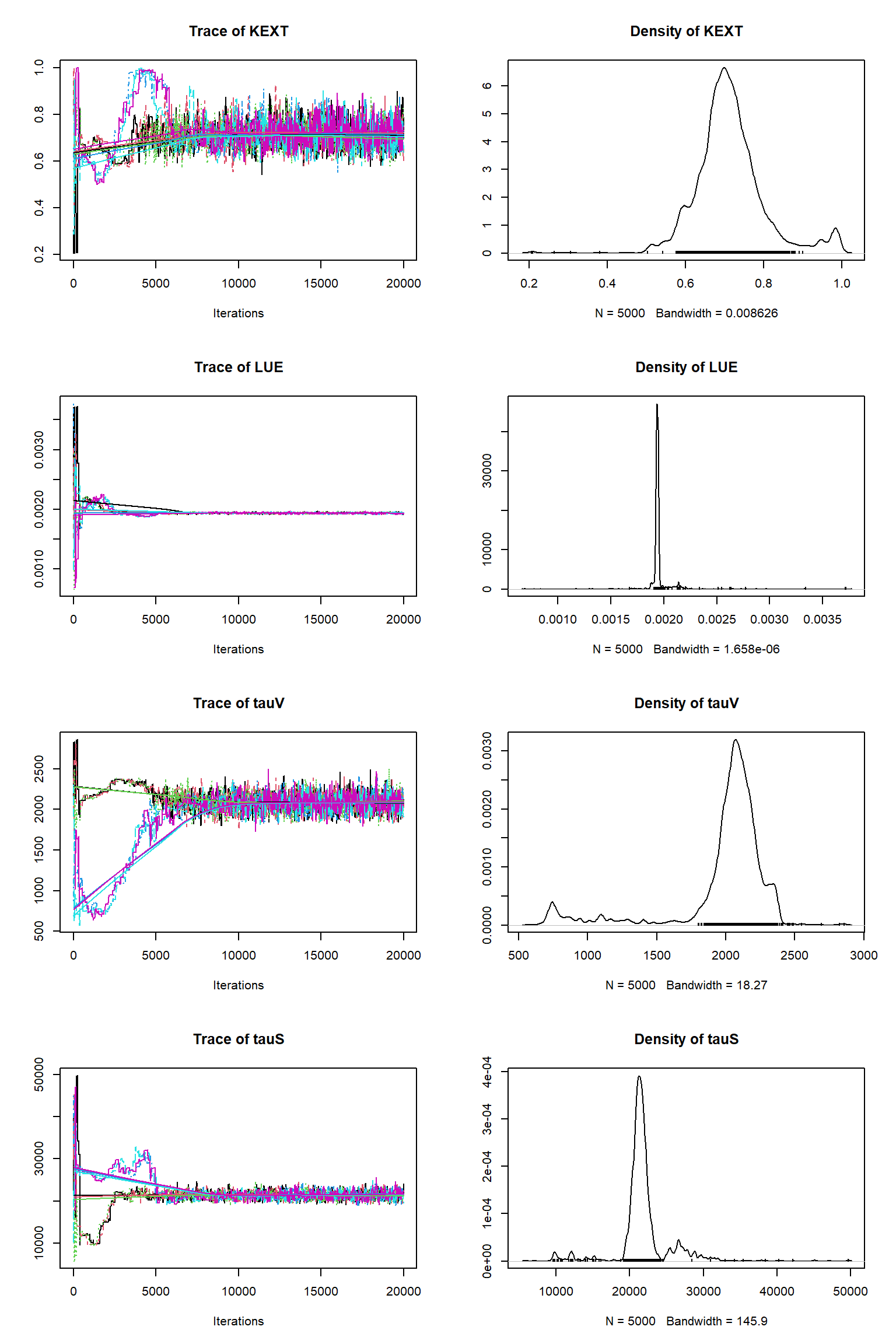
bout = getSample(out,thin=10,start=15000)
tracePlot(sampler = bout)
ifld<-2
myObs<-obs[,ifld]
myObs[-obsSel] <- NA
plotTimeSeriesResults(sampler = bout, model = createPredictions, observed = myObs,
                      plotResiduals=FALSE, error = createError, prior = FALSE, main = "Cv posterior predictive")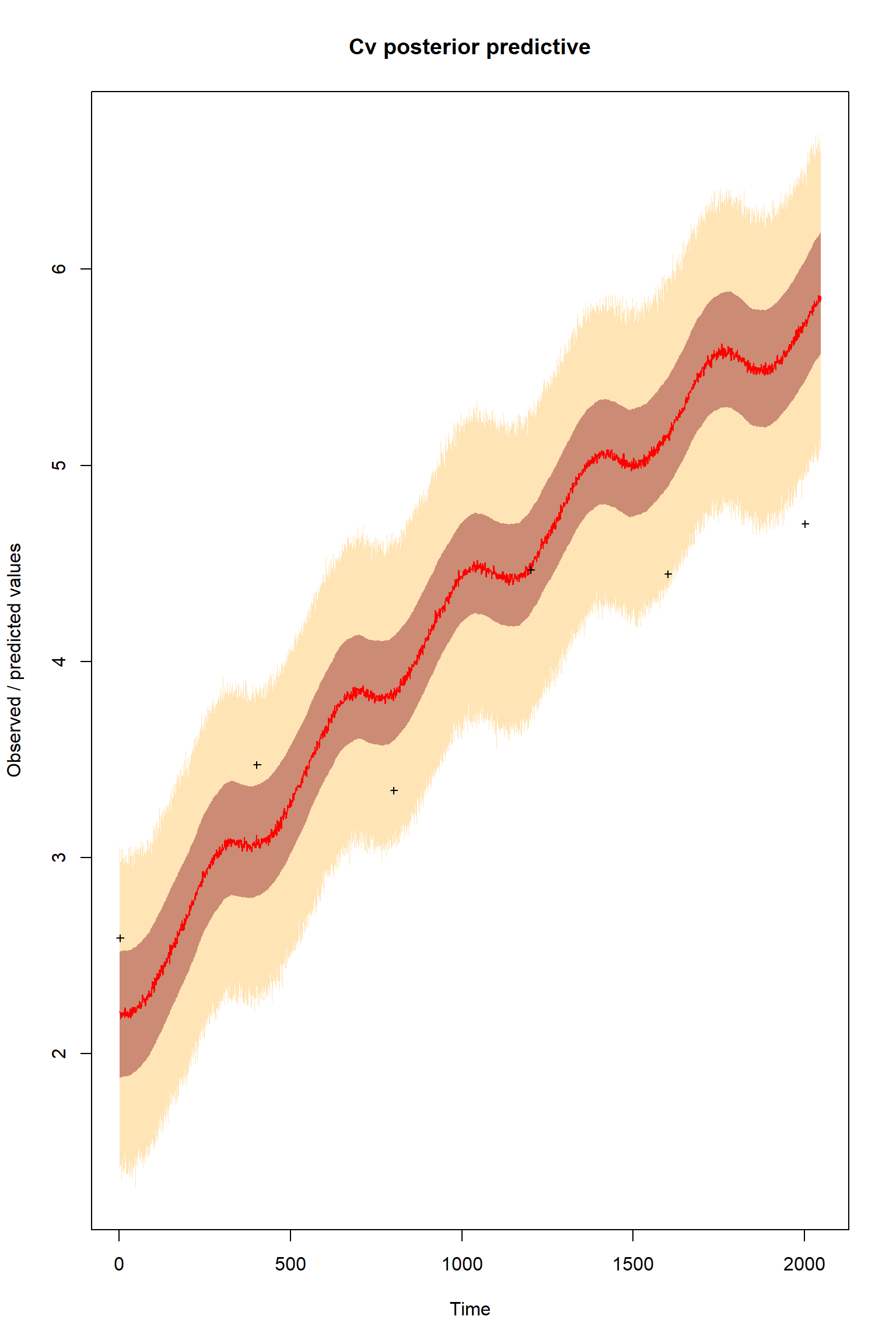
ifld<-3
myObs<-eobs
plotTimeSeriesResults(sampler = bout, model = createPredictions, observed = myObs,
                      plotResiduals=FALSE, error = createError, prior = FALSE, main = "Cs posterior predictive")
Questions
These results are remarkably similar to the previous inference with a model structural error and an imbalanced dataset. What does this suggest?
Modifying the log likelihood function to express our uncertainty about observational bias
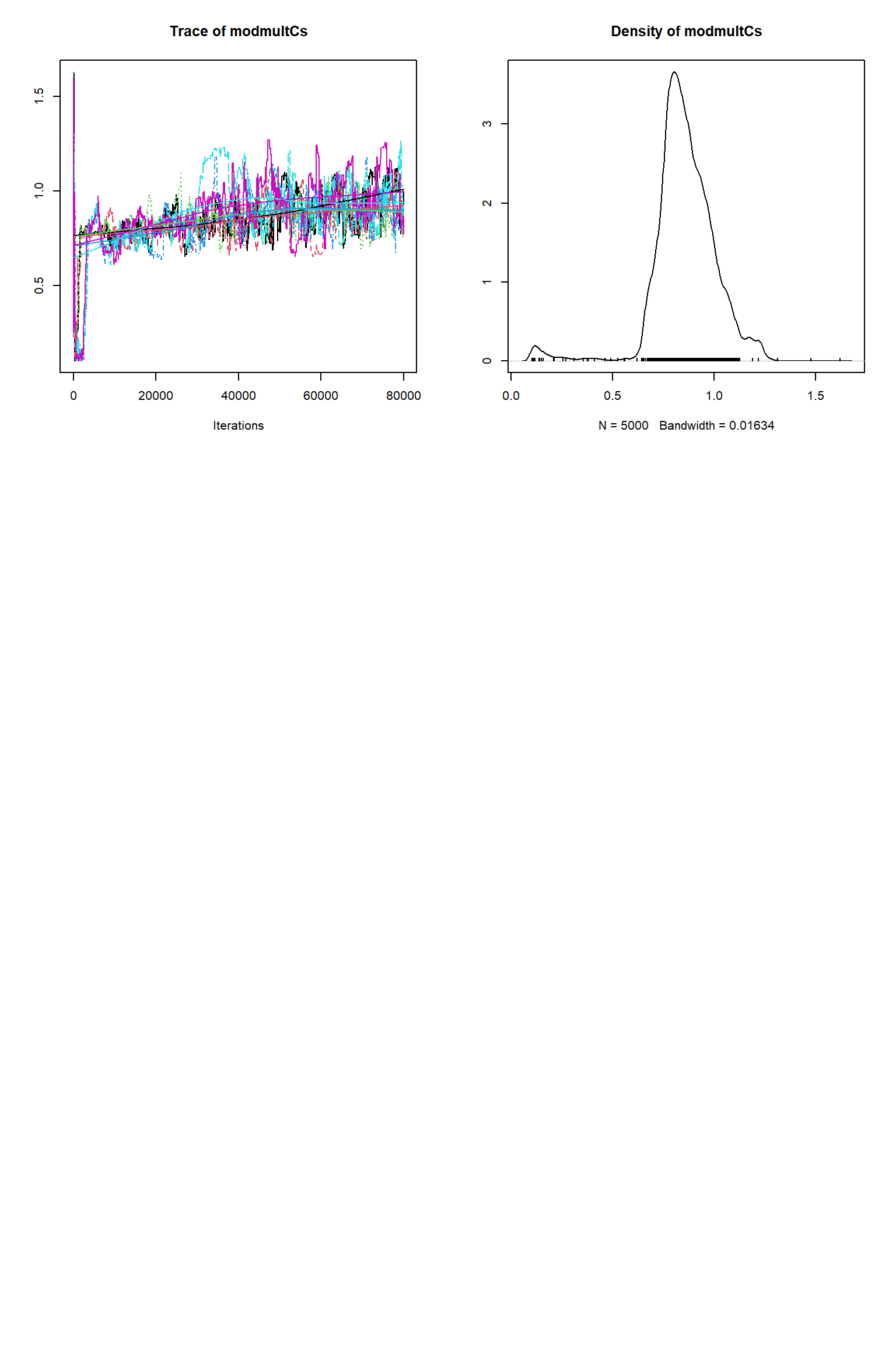
The issues with the inferences above isn’t the presence of model or observational error or indeed imbalances in data. Rather it is that we have not been representing our unceratainties in these errors in the inference. Here we have added linear multiplication terms as uncertain parameters in the log likelihood function to express our uncertainty about the size and presence of a systematic bias in the observational data. This adds three more parameters to the inference and so necessitates a significantly longer chain before convergence. To speed things up given the time that we have I have included the output from an inference I made previously so that we won’t have to wait for the inference to finish.
addPars                   <- refPars
nvar                      <- length(addPars$best)

addPars[nvar+1,]          <- c(1.0, 0.1, 2.0)
addPars[nvar+2,]          <- c(1.0, 0.1, 2.0)
addPars[nvar+3,]          <- c(1.0, 0.1, 2.0)
rownames(addPars)[nvar+1]   <- "modmultNEE"
rownames(addPars)[nvar+2]   <- "modmultCv"
rownames(addPars)[nvar+3]   <- "modmultCs"
nparSel <- c(parSel, nvar+1,nvar+2,nvar+3)

obsSel=seq(2,2048,400)

likelihood <- function(par, sum = TRUE){
  # set parameters that are not inferred to default values
  x = addPars$best
  x[nparSel] = par
  predicted <- VSEM(x[1:11], PAR) # replace here VSEM with your model
  predicted[,1] = 1000 * predicted[,1] # this is just rescaling

  diff       <- c(predicted[,1]*x[nvar+1] - obs[,1])
  llValues1  <- dnorm(diff, sd = x[nvar]*(maobs[1]), log = T)
  diff <- c(( predicted[1,2] + (predicted[obsSel,2] - predicted[1,2])*x[nvar+2] ) - obs[obsSel,2])
  llValues2  <- dnorm(diff, sd = x[nvar]*maobs[2], log = T)
  diff <- c(( predicted[1,3] + (predicted[,3] - predicted[1,3])*x[nvar+3] ) - eobs)
  llValues3  <- dnorm(diff, sd = x[nvar]*maobs[3], log = T)

  return(sum(llValues1,llValues2,llValues3))
}


# optional, you can also directly provide lower, upper in the createBayesianSetup, see help
prior <- createUniformPrior(lower = addPars$lower[nparSel],
                            upper = addPars$upper[nparSel], best = addPars$best[nparSel])

bayesianSetup <- createBayesianSetup(likelihood, prior, names = rownames(addPars)[nparSel])

# settings for the sampler, iterations should be increased for real applicatoin
settings <- list(iterations = 240000, nrChains = 2)

#out <- runMCMC(bayesianSetup = bayesianSetup, sampler = "DEzs", settings = settings)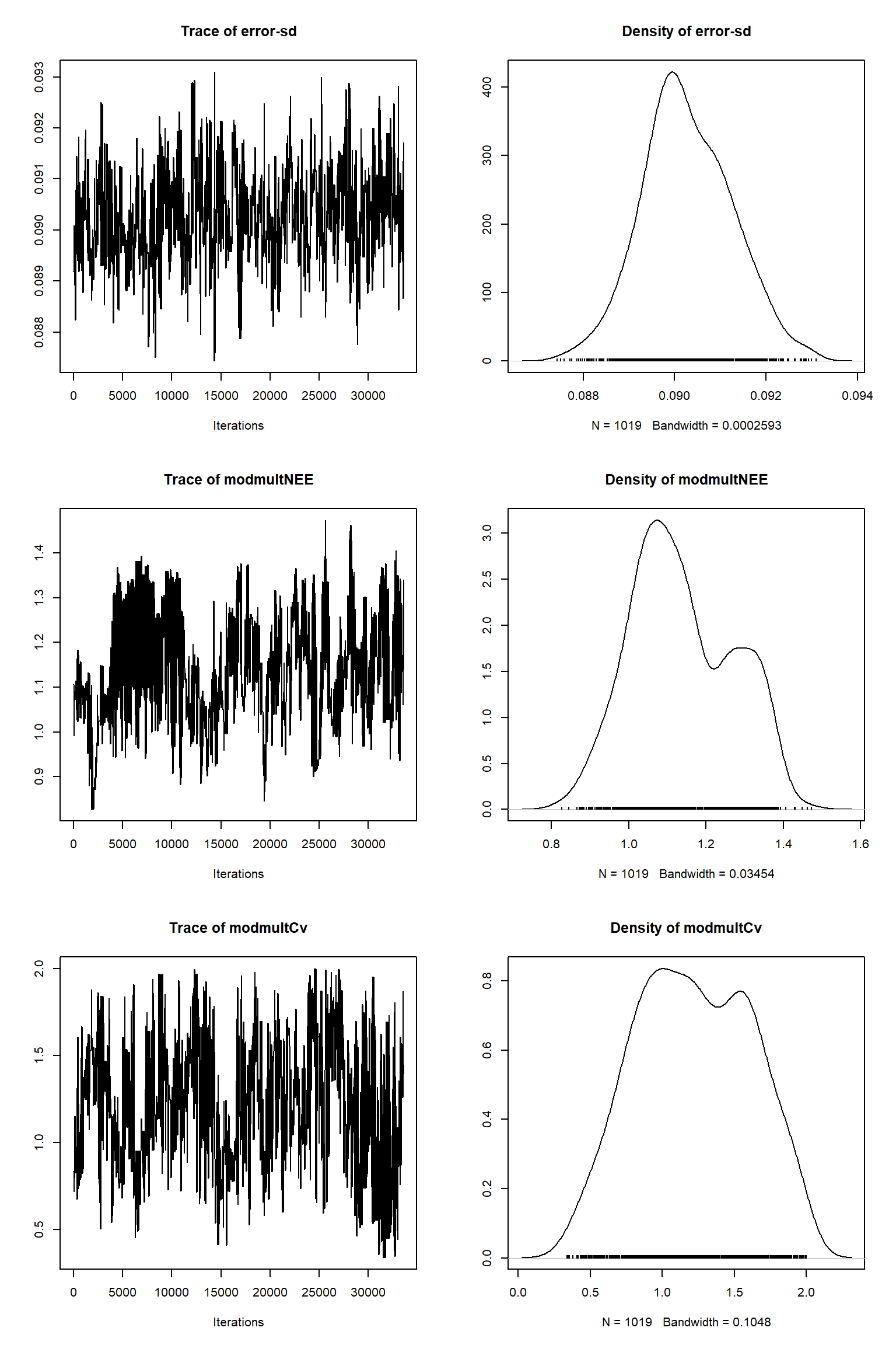
out = readRDS(file= url("https://raw.githubusercontent.com/NERC-CEH/beem_data/main/vsem-chain240k.rds"))tracePlot(sampler = out)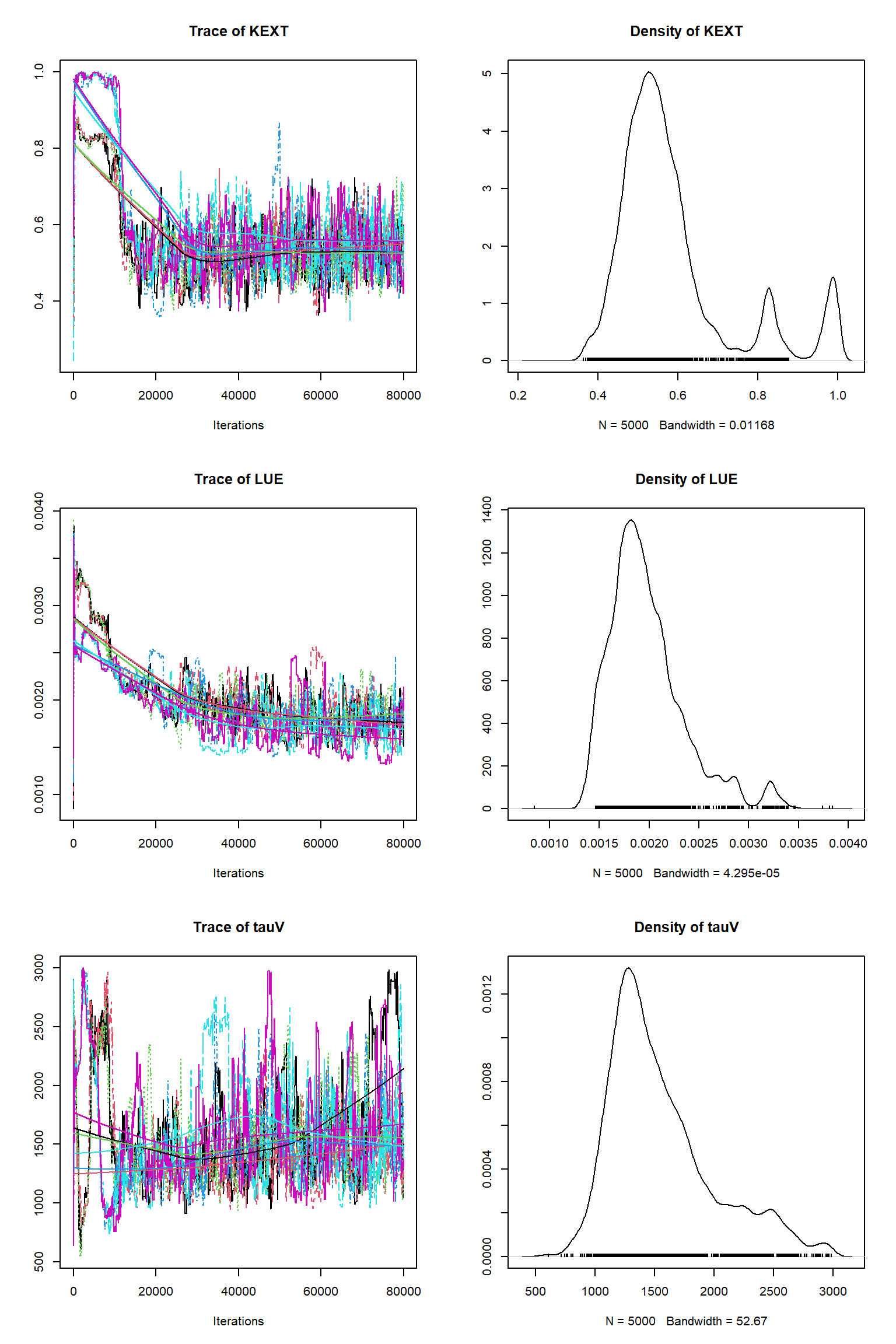
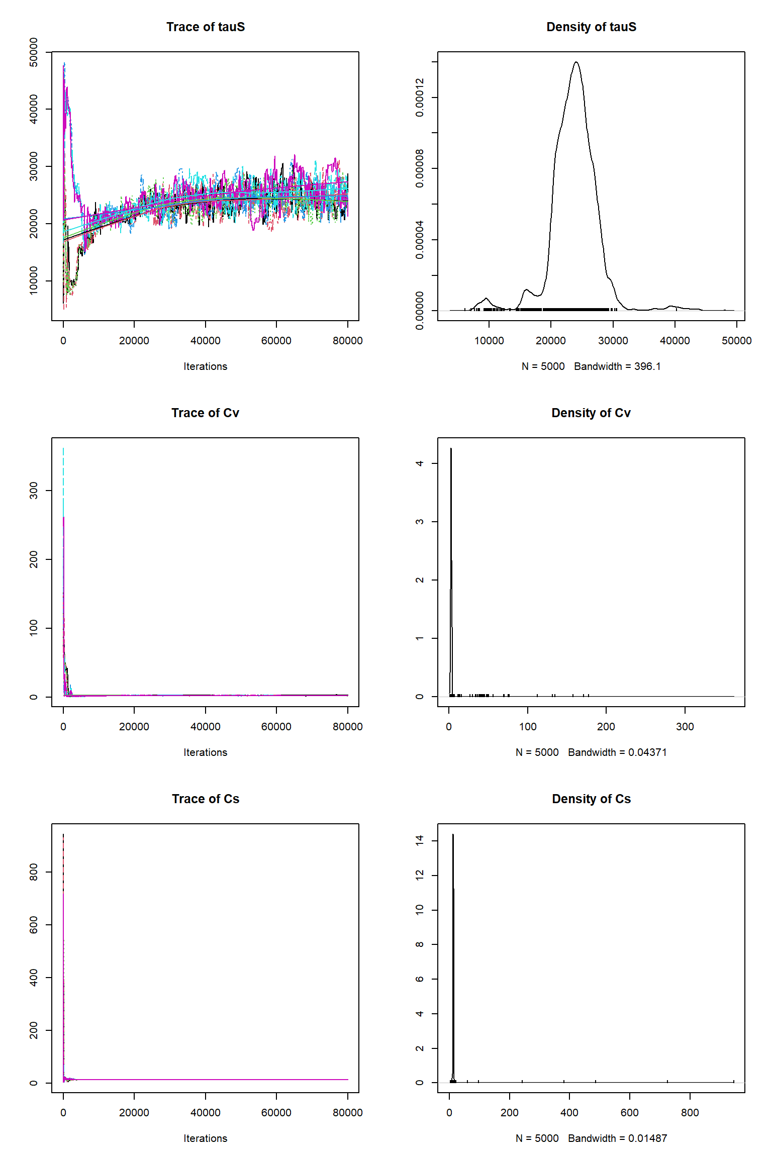
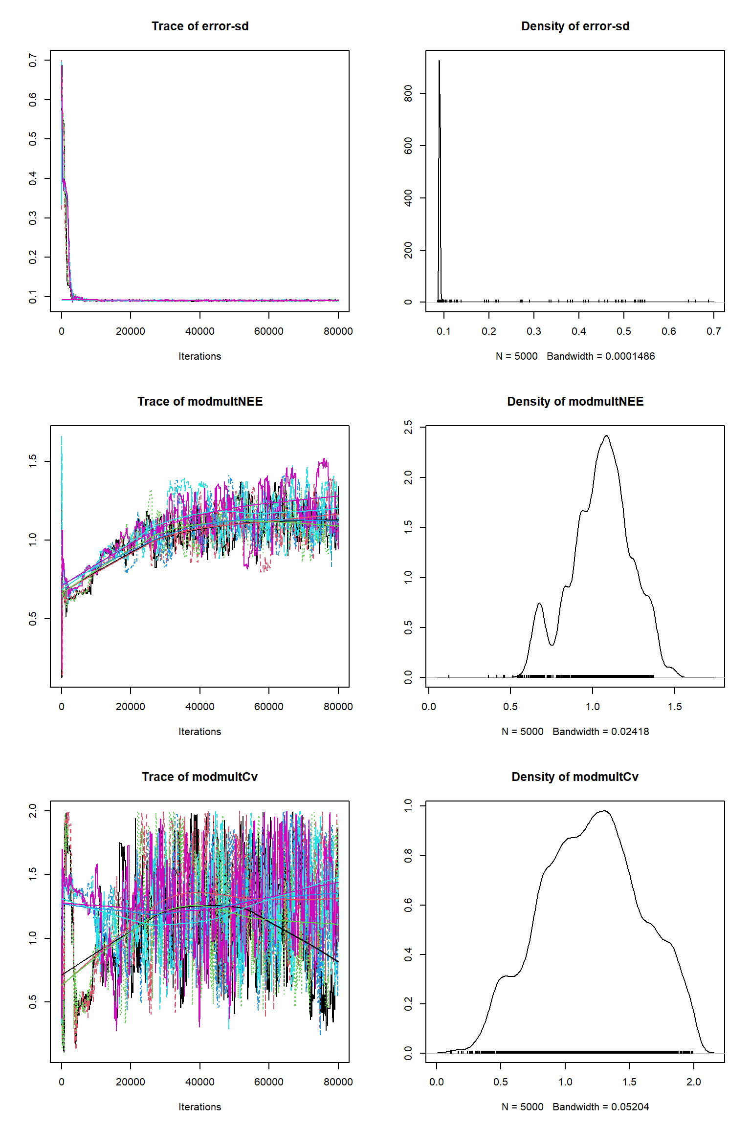
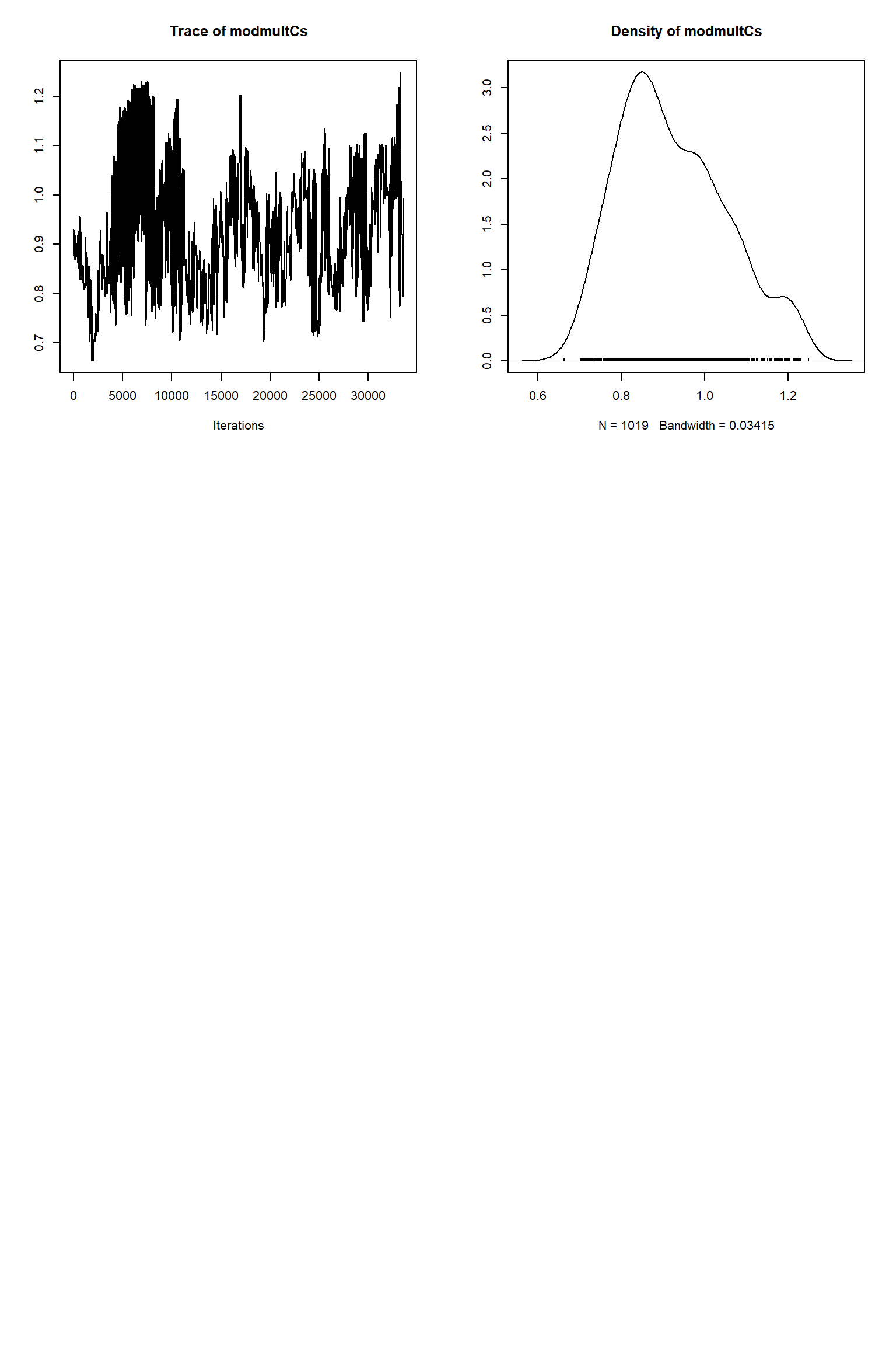
bout = getSample(out,thin=10,start=24000)
tracePlot(sampler = bout)
createPredictionsmodL <- function(par){
  # set the parameters that are not inferred to default values
  x = addPars$best
  x[nparSel] = par
  predicted <- VSEM(x[1:11], PAR) # replace here VSEM with your model
  predicted[,1] = predicted[,1] * 1000
  predicted[,ifld] <- ( predicted[1,ifld] + (predicted[,ifld] - predicted[1,ifld])*x[nvar+ifld] )
  return(predicted[,ifld])
}

ifld<-2
myObs<-obs[,ifld]
myObs[-obsSel] <- NA
plotTimeSeriesResults(sampler = bout, model = createPredictionsmodL, observed = myObs,
                      plotResiduals=FALSE, error = createError, prior = FALSE, main = "Cv posterior predictive")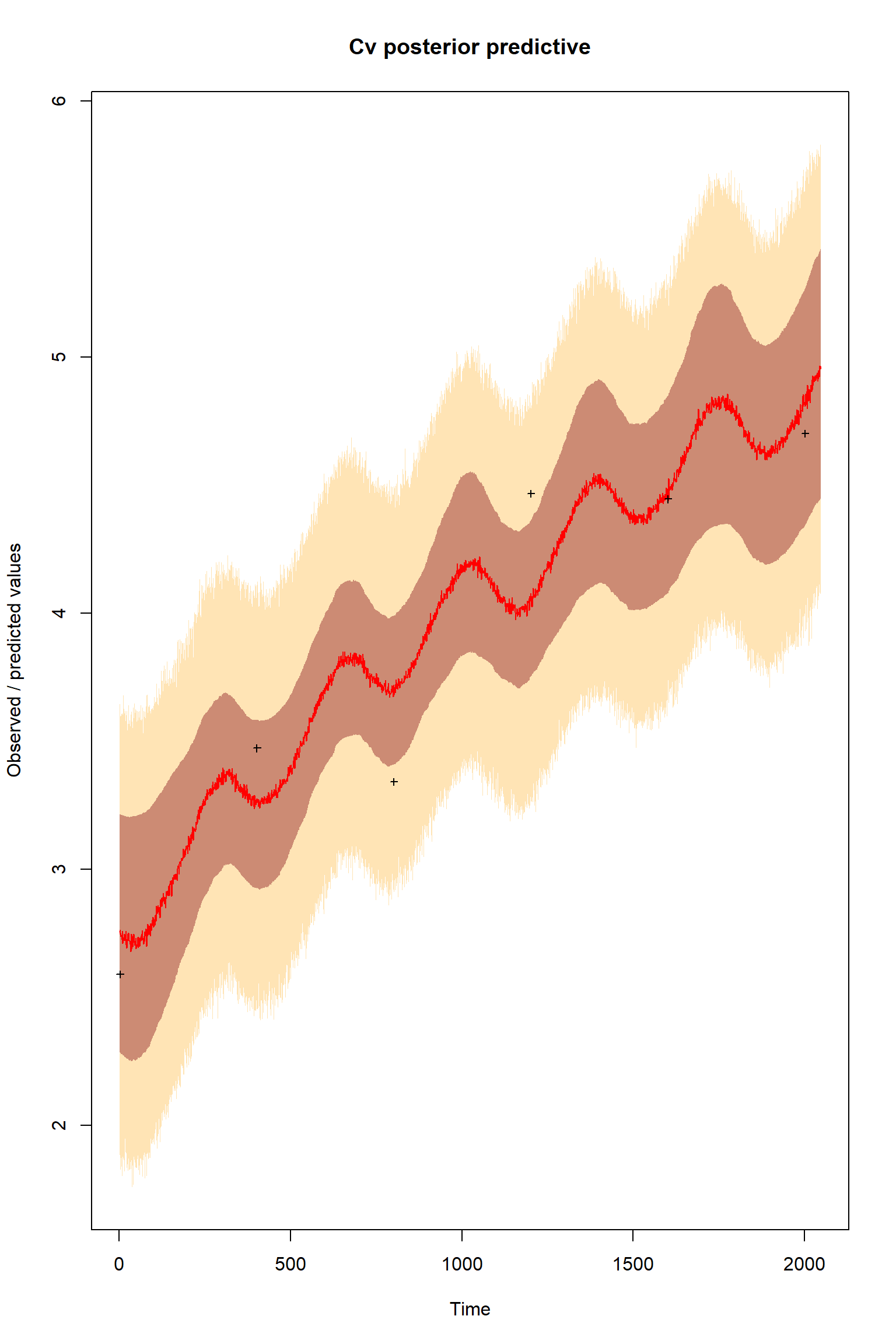
ifld<-3
myObs<-eobs
plotTimeSeriesResults(sampler = bout, model = createPredictionsmodL, observed = myObs,
                      plotResiduals=FALSE, error = createError, prior = FALSE, main = "Cs posterior predictive")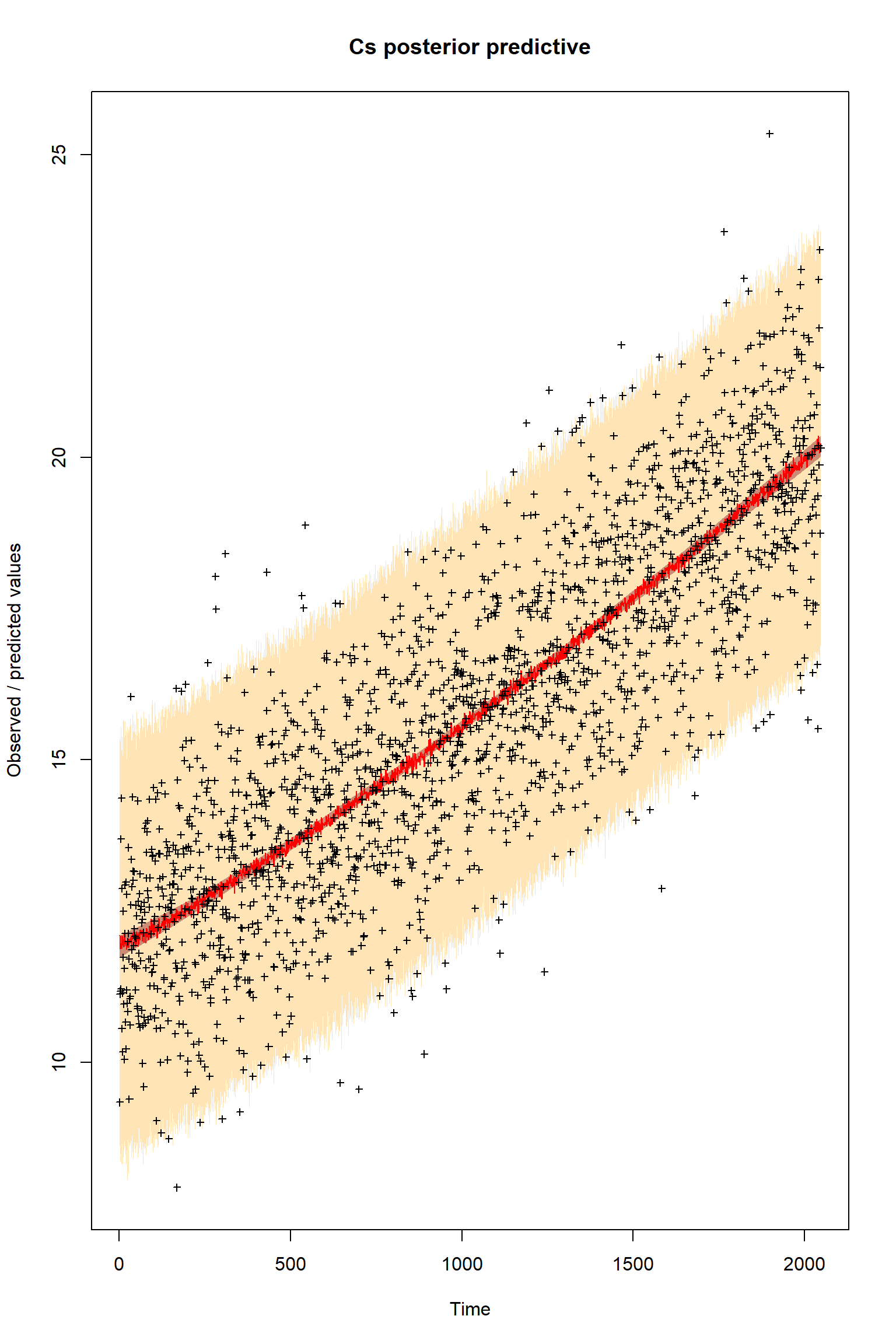
Questions
There is a good fit to the observations after this inference. Have a look at the marginal parameter distributions. What do you notice about them? Is there any improvement over previous inferences? Compare the posterior Cv plot with the one from the first inference where there were no systematic errors present and the quantities of data were balanced - what differences do you notice and why do you think they are different?
Representing uncertainty about model/data errors in Bayesian Inference of PBMs
Here we were able to make a good choice in representing our uncertainty in the systematic bias in the observations. Normally we do not know much about any model structural errors or observational systematic biases that may be present. Our uncertainty about these errors make it challenging to represent them well in inferences. This remains one of the main challenges in infering the parameters of process-based ecological models. Yet it is crucially important to be aware of these issues, hence the reason that we have focussed on them in this practical. To read more about this see our recent publication (Cameron et al 2023).
References
Cameron, D., Hartig, F., Minnuno, F., Oberpriller, J., Reineking, B., Van Oijen, M., & Dietze, M. (2022). Issues in calibrating models with multiple unbalanced constraints: the significance of systematic model and data errors. Methods in Ecology and Evolution, 13, 2757–2770. https://doi.org/10.1111/2041-210X.14002