Bayesian Methods for Ecological and Environmental Modelling
Author
Peter Levy
Bayesian machine learning
In this practical, we will use the R package BART as an example of a probabilistic machine learning method. We will use the tree allometry dataset we have seen earlier, but this time we will attempt to predict the mass of roots of each tree (the variable root_mass).
Read the dataset. You could create some basic ggplot2 or GGally plots to check the distribution of root_mass and the relationships between root_mass and other variables such as age, cultivation, tree_height, and species.
# Load the required librarylibrary(BART)
Warning: package 'BART' was built under R version 4.4.3
Loading required package: nlme
Loading required package: survival
library(ggplot2)
Warning: package 'ggplot2' was built under R version 4.4.3
library(tidyr)
Warning: package 'tidyr' was built under R version 4.4.3
# Set a seed for reproducibility of random numbersset.seed(123)# Read the datadf <-read.csv(url("https://raw.githubusercontent.com/NERC-CEH/beem_data/main/trees.csv"))# remove missing valuesdf <-na.omit(df)names(df)
# GGally makes a nice plot but too big for the web page# library(GGally)# GGally::ggpairs(df)
BART cannot cope with factor or character variables, so convert the factors into numeric variables.
# convert character variables to integers df$species <-as.integer(as.factor(df$species))df$soil_type <-as.integer(as.factor(df$soil_type))
Converting to integers is not really sensible - better to “one-hot” encoding i.e. columns of 1s and 0s, but this would make a larger data frame that we want for demo purposes. Here we use the integer version of species to produce a deliberately bad linear model. It is also common to scale all variables and apply transformations (such as log) when things are very skewed, but we skip that for now.
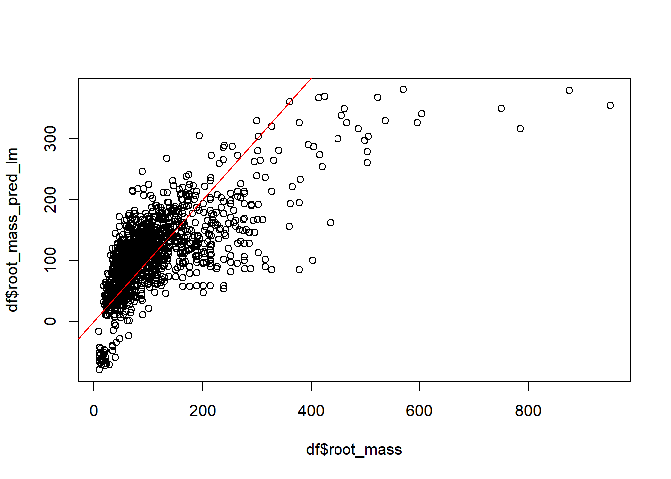
First, we establish a simple linear model, fitted by ordinary least squares, which we design to give a poor linear fit - we leave out some obvious predictors (tree_mass, dbh), and add in species which should not give a linear response.
m <-lm(root_mass ~ age + cultivation + tree_height + species, data = df)summary(m)
Call:
lm(formula = root_mass ~ age + cultivation + tree_height + species,
    data = df)

Residuals:
    Min      1Q  Median      3Q     Max
-157.22  -38.87  -12.42   22.82  596.02

Coefficients:
             Estimate Std. Error t value Pr(>|t|)
(Intercept) -220.5058    11.0783 -19.904  < 2e-16 ***
age            1.5718     0.3068   5.124 3.43e-07 ***
cultivation   -1.1513     0.7143  -1.612    0.107
tree_height   17.0161     0.6675  25.491  < 2e-16 ***
species        5.2628     0.5619   9.367  < 2e-16 ***
---
Signif. codes:  0 '***' 0.001 '**' 0.01 '*' 0.05 '.' 0.1 ' ' 1

Residual standard error: 65.19 on 1355 degrees of freedom
Multiple R-squared:  0.4879,    Adjusted R-squared:  0.4864
F-statistic: 322.8 on 4 and 1355 DF,  p-value: < 2.2e-16
To fit a machine learning model, we have to split the data into training and test sets. These models can be quite slow, and reducing the fraction used as the training proportion will speed things up.
# Split the data into training and test sets (70% training, 30% testing)train_index <-sample(1:nrow(df), 0.7*nrow(df))df_train <- df[train_index, ]df_test <- df[-train_index, ]# Defining the response and covariates for trainingy.train <- df_train$root_mass# x.train <- as.matrix(df_train[, c("dbh", "tree_height")])# x.train <- as.matrix(df_train[, c("age", "cultivation", "tree_height", "taper", "dbh")])x.train <-as.matrix(df_train[, c("age", "cultivation", "tree_height", "species")])# Defining the covariates for testing# x.test <- as.matrix(df_test[, c("dbh", "tree_height")])# x.test <- as.matrix(df_test[, c("age", "cultivation", "tree_height", "taper", "dbh")])x.test <-as.matrix(df_test[, c("age", "cultivation", "tree_height", "species")])
Fit BART model to the training data using the wbart function. Behind the scenes, it runs MCMC chains using the Metropolis-Hastings algorithm. It thereby estimate the posterior distribution of the regression tree parameters.
*****Into main of wbart
*****Data:
data:n,p,np: 951, 4, 409
y1,yn: -52.696058, -5.896058
x1,x[n*p]: 24.000000, 11.000000
xp1,xp[np*p]: 44.000000, 11.000000
*****Number of Trees: 200
*****Number of Cut Points: 29 ... 11
*****burn and ndpost: 100, 1000
*****Prior:beta,alpha,tau,nu,lambda: 2.000000,0.950000,15.322178,3.000000,752.802698
*****sigma: 62.166387
*****w (weights): 1.000000 ... 1.000000
*****Dirichlet:sparse,theta,omega,a,b,rho,augment: 0,0,1,0.5,1,4,0
*****nkeeptrain,nkeeptest,nkeeptestme,nkeeptreedraws: 1000,1000,1000,1000
*****printevery: 100
*****skiptr,skipte,skipteme,skiptreedraws: 1,1,1,1

MCMC
done 0 (out of 1100)
done 100 (out of 1100)
done 200 (out of 1100)
done 300 (out of 1100)
done 400 (out of 1100)
done 500 (out of 1100)
done 600 (out of 1100)
done 700 (out of 1100)
done 800 (out of 1100)
done 900 (out of 1100)
done 1000 (out of 1100)
time: 10s
check counts
trcnt,tecnt,temecnt,treedrawscnt: 1000,1000,1000,1000
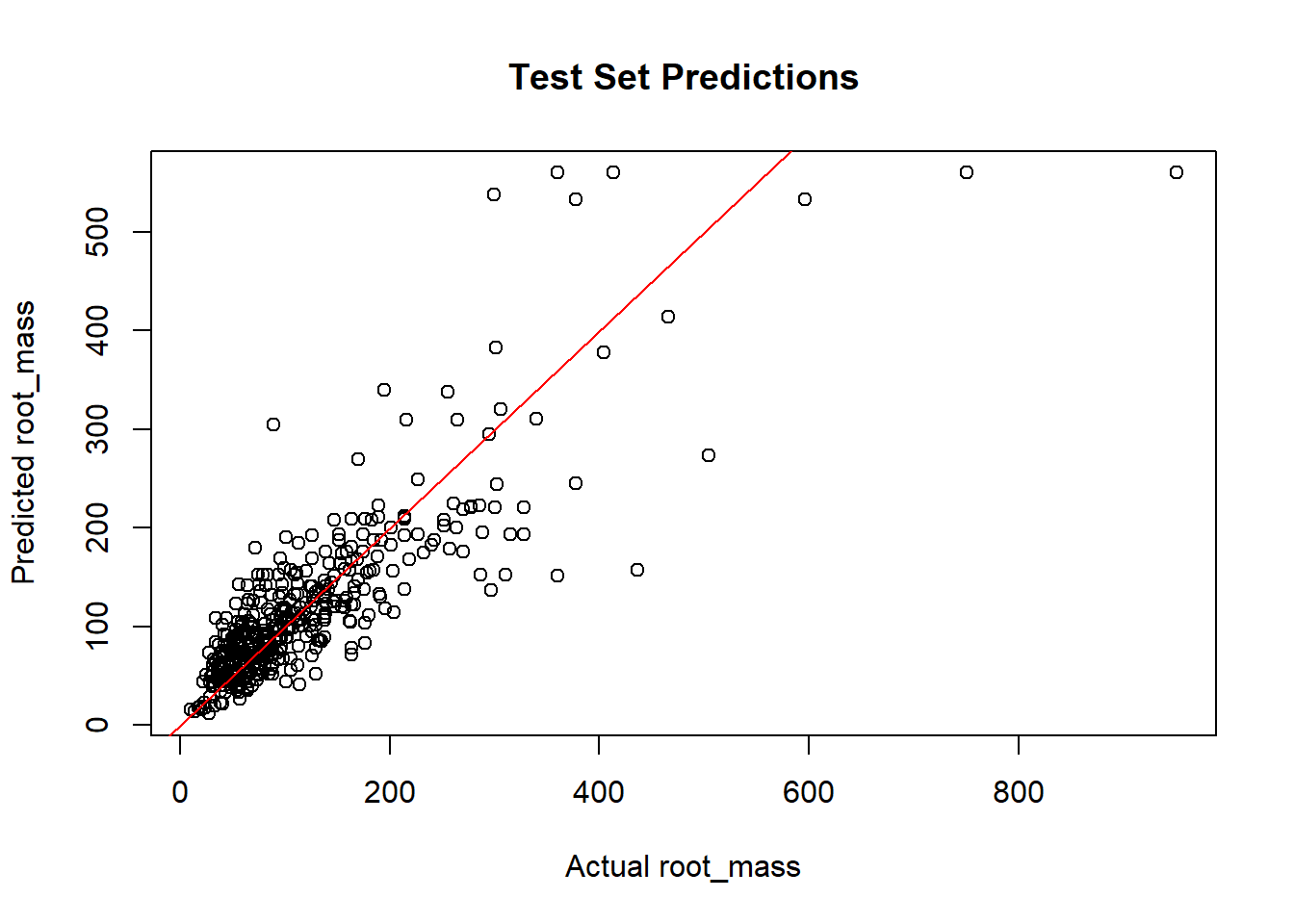
Evaluate the performance of the BART model using the Root Mean Squared Error (RMSE) on the test set. We then add some code to predict the root mass in the test set using the fitted BART model.
# Plotting the fitted BART model# Extracting the test set predictionstest_predictions <- bart_model$yhat.test.mean# RMSE(rmse <-sqrt(mean((test_predictions - df_test$root_mass)^2)))
[1] 54.06613
# Plot the the fitted BART model predictions for the test setplot(df_test$root_mass, test_predictions, xlab="Actual root_mass", ylab="Predicted root_mass",main="Test Set Predictions")abline(0, 1, col="red")
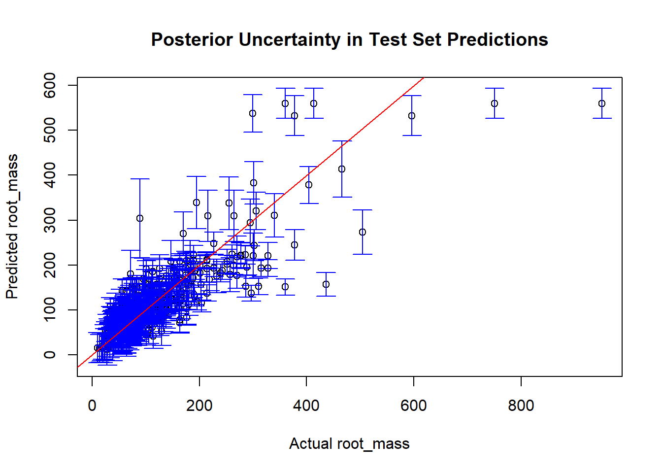
You can extract the full posterior distribution of predictions. We create a 95% interval for each row in the test set and produce a plot of true vs predicted values.
# Plotting the posterior uncertainty in the test set predictionsposterior_predictions <-t(bart_model$yhat.test)posterior_mean <-rowMeans(posterior_predictions)df_test$root_mass_pred_bart <-rowMeans(posterior_predictions)posterior_sd <-apply(posterior_predictions, 1, sd)# Create 95% confidence intervalsposterior_low <- posterior_mean -1.96* posterior_sdposterior_high <- posterior_mean +1.96* posterior_sd# Now show the uncertaintyplot(df_test$root_mass, posterior_mean, ylim =range(c(posterior_low, posterior_high)),xlab="Actual root_mass", ylab="Predicted root_mass",main="Posterior Uncertainty in Test Set Predictions")arrows(df_test$root_mass, posterior_low, df_test$root_mass, posterior_high,angle=90, code=3, length=0.1, col="blue")abline(0, 1, col ='red')
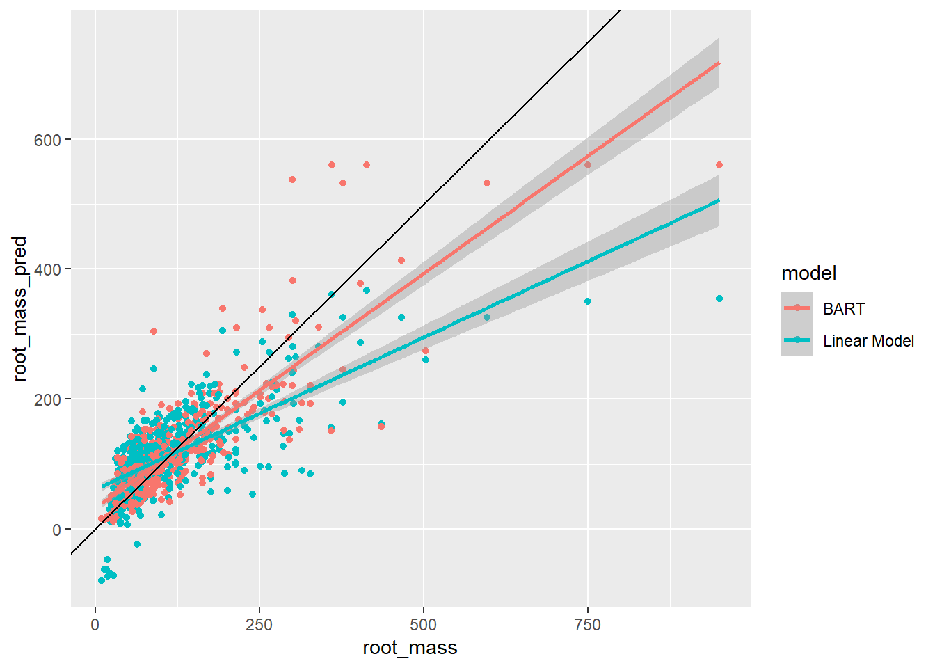
Compare this with the simple linear model fitted earlier. We create a plot using ggplot2 of the predicted values vs the true values for both models.
df_test$root_mass_pred_lm <-predict(m, newdata = df_test)# reshape to long format for ggplotdf_test <-pivot_longer(df_test, cols =c("root_mass_pred_lm", "root_mass_pred_bart"), names_to ="model", values_to ="root_mass_pred")# give sensible namesdf_test$model[df_test$model =="root_mass_pred_lm"] <-"Linear Model"df_test$model[df_test$model =="root_mass_pred_bart"] <-"BART"p <-ggplot(df_test, aes(root_mass, root_mass_pred, colour = model))p <- p +geom_point()p <- p +stat_smooth(method ="lm")p <- p +geom_abline()p
`geom_smooth()` using formula = 'y ~ x'
Questions:
Does the BART model give a closer fit to the data?
How sensitive are the results to the number of trees used (ntree argument in wbart)?
Try using different numbers of predictor (\(x\)) variables in the model. When does BART give an advantage?