Lake water quality example: Esthwaite Water, UK
What is adatpive sampling?
Adpative sampling is the opposite of sampling with a fixed design. A majority of previous adaptive sampling is applied spatially, where collected data determined the spatial location of the samples in the next sampling round. Here we focus on temporal adatpive sampling, where sampling frequencies effectively changes based on measured data or other information.
The multi-rule approach
Adaptive sampling means sampling that goes beyonds fixed designs of sampmling at regular intervals. In practice, changing sampling frequencies all the time can lead to a variety of issues. Therefore, using a combination of multiple rules, each sampling at regular intervals and activated by different criteria, to achieve adaptive sampling is more flexible and is preferred.
| Multi-rule adaptive sampling (this R package) | Dynamic frquency adaptive sampling |
|---|---|
| Each rule samples at regular intervals, but are triggered adaptively. | Sampling frequencies can change abruptly and unexpeectedly. |
| The combination of rules make the approach highly flexible. | More challenging to analyze data. |
| You can analyze data from each rule separately. | |
| Baseline data for trend monitoring will not be disrupted. | |
| Ideal solution to combine compliance monitoring with taking opportunisitc measurements. |
Example data: Esthwaite lake monitoring data and SUNA nitrate sensor
For demonstration, we use field trial data from in-lake physico-chemical sensors (water temperature at 12 depths, and Ponsel temperature and conductivity), over-lake weather sensors (air temperature, wind speed, wind direction, solar radiation, relative humidity) sonde and a SUNA optical nitrate sensor on an automatic buoy located on Esthwaite water in Lake District, England collected between 29th April to 22nd October 2025. Optical nitrate data was collected every 10 minutes, while the other determinants are measured at every 2 minutes. While no specific events are expected in this lake, we use this dataset to demonstrate the various techniques for adaptive sampling.
Evaluation: some metrics
Following Elfferich et al. (2024), we will report the median and range captured by the downsampled time series, which is applicable to adaptively sampled time series in retrospective experiments. is the orginal time series, while is the sub-sampled time series.
Percentage of range captured
Percentage change of median
Loading libraries
Loading data
The following data has been loaded in the adaptNP R package.
# filepath <- 'temp/Esthwaite_Buoy_Data_May_to_Oct_2025.xlsx'

# excel_sheets(filepath)

# # print header
# print( read_excel(filepath, sheet = "Esthwaite_Buoy_HiRes", n_max = 0))

# Esthwaite_Buoy_HiRes <- read_excel(filepath, sheet = "Esthwaite_Buoy_HiRes", skip=1) # every 2 minutes

# # print header
# print( read_excel(filepath, sheet = "Esthwaite_Buoy_SUNA_Data", n_max = 0))

# Esthwaite_Buoy_SUNA_Data <- read_excel(filepath, sheet = "Esthwaite_Buoy_SUNA_Data", skip=1) # every 10 minutes
Example 1: threshold rules
We will illustrate the method by using a simple rule:
criteria <-"(Temp4m > 18) | (SPFD >800)"
The adapt-NP R package make it very easy to do so.
- The
flag_eventfunction returns whether or not the criterion is met (i.e. a event). - The
extract_event_periodsfunction extract periods (i.e. dictionary of start and end times) where the event occurs. Note you can specify to extract only events that are longer than a particular duration (specifically, number of records).
criteria <-"(Temp4m > 18) | (SPFD >800)"

# flag event (True or false)
Esthwaite_Buoy_HiRes <- flag_event(Esthwaite_Buoy_HiRes,criteria)

# extract event periods (i.e. start and end)
periods  <- extract_event_periods(
  Esthwaite_Buoy_HiRes %>%
    rename(timestamp=TIMESTAMP,flag=event_flag)  |> tidyr::drop_na(flag),
  min_length=50)

# convert period to R lubridate intervals
intervals <- periods |>
  mutate(int = interval(start,end) ) |>
  pull(int)
After extracting the event periods, the following code snippets uses it to subset the dataset.
# rule 0: every 6h
baseline <- Esthwaite_Buoy_SUNA_Data |>
  select(TIMESTAMP, SUNA_Nitrate_mgL) |>
  mutate(hour = lubridate::hour(TIMESTAMP),
         minute = lubridate::minute(TIMESTAMP)) |>
  filter(minute==0, hour %in% c(3,9,15,21))

# rule 1: every 10 or 20 minutes within periods

# very fast!
mask <- Reduce(`|`, lapply(intervals, function(int) Esthwaite_Buoy_SUNA_Data$TIMESTAMP %within% int))
rule1 <- Esthwaite_Buoy_SUNA_Data[mask, ]
Now, we plot the results.
# now plot: (1) all SUNA, (2) baseline SUNA, (3) rule 1 SUNA

combined_SUNA <- Esthwaite_Buoy_SUNA_Data |> select(TIMESTAMP, SUNA_Nitrate_mgL) |>
  left_join(rule1 |> select(TIMESTAMP, SUNA_Nitrate_mgL) |> rename(rule1 = SUNA_Nitrate_mgL), by='TIMESTAMP') |>
  left_join(baseline |> select(TIMESTAMP, SUNA_Nitrate_mgL) |> rename(baseline = SUNA_Nitrate_mgL), by='TIMESTAMP')

anno <- data.frame(xtext = c('2025-07-15', '2025-07-15', '2025-07-15'),
                   ytext = c(0.4,0.4,0.4),
                   Rule = c("raw data", "rule 0 (baseline)" ,"rule 1 (algal bloom likely)" ),
                   text = c("Every 10 minutes", "Every 6 hours", "Every 10 minutes only during event")) |>
  mutate(xtext = as.Date(xtext))

combined_SUNA |>
  rename( `raw data` = SUNA_Nitrate_mgL,
          `rule 0 (baseline)` = baseline,
          `rule 1 (algal bloom likely)` = rule1,) |>
#  filter(TIMESTAMP <'2025-08-15') |>
  tidyr::pivot_longer(!TIMESTAMP, names_to = "Rule", values_to = "value") |>
  ggplot2::ggplot() +
  geom_point(aes(x = TIMESTAMP, y=value, colour = factor(Rule))) +
  facet_grid(rows = vars(Rule)) +
  # scale_fill_manual(values = c("red", "blue", "green")) +
  scale_color_manual(
    name   = "",                      # legend title
    values = c("raw data" = "#000000",
               "rule 0 (baseline)" = "#1b9e77",
               "rule 1 (algal bloom likely)" = "#d95f02")
  ) +
    geom_text(data = anno, aes(x = xtext,  y = ytext, label = text), size=5) +
  theme_gov() +
#   geom_rect(data = periods |> mutate(start=as.Date(start), end=as.Date(end)),
#             aes(xmin = start, xmax = end, ymin = -Inf, ymax = Inf),
#             fill = "lightpink", alpha= 0.3)+
  theme(legend.position='bottom',
        panel.spacing = unit(2, "lines"),
        text=element_text(size=20), #change font size of all text
        # axis.line = element_line(linewidth = 3, colour = "grey20"),
        strip.background = element_blank(),
        strip.text.y = element_blank(),
        axis.text=element_text(size=20), #change font size of axis text
        axis.title=element_text(size=20), #change font size of axis titles
        plot.title=element_text(size=16), #change font size of plot title
        legend.text=element_text(size=20), #change font size of legend text
        legend.title=element_text(size=20))+ #change font size of legend title
  ggtitle('2025 SUNA nitrate sensor field trial, Esthwaitewater, UK \n') +
  labs(x='',y='mg/L')+ ylim(0,0.5) +
  guides(colour = guide_legend(override.aes = list(size=8))) # change legend point size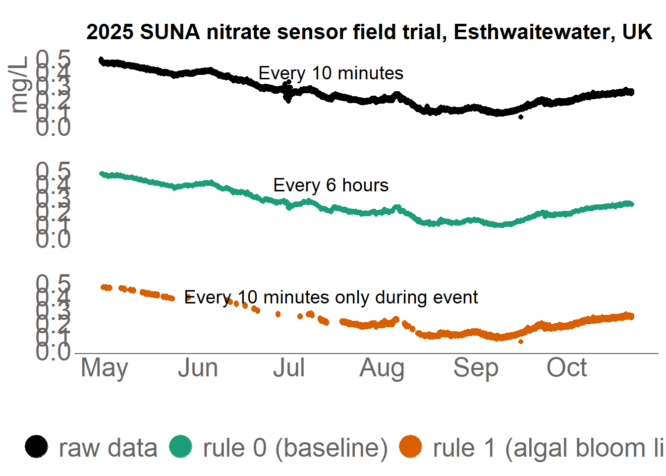
# plot periods (hours flagged per day) as rectangles: y axis (date), x axis (hours)
periods  |> mutate(duration = interval(start,end)%/%minutes(1))
start end duration
1 2025-04-30 09:34:00 2025-04-30 15:18:00 344
2 2025-05-01 08:30:00 2025-05-01 12:26:00 236
3 2025-05-01 12:44:00 2025-05-01 16:02:00 198
4 2025-05-02 09:24:00 2025-05-02 11:08:00 104
5 2025-05-02 11:24:00 2025-05-02 13:30:00 126
6 2025-05-02 14:34:00 2025-05-02 16:14:00 100
7 2025-05-06 08:20:00 2025-05-06 10:58:00 158
8 2025-05-07 08:14:00 2025-05-07 11:06:00 172
9 2025-05-07 12:34:00 2025-05-07 14:16:00 102
10 2025-05-09 08:28:00 2025-05-09 14:26:00 358
11 2025-05-09 14:34:00 2025-05-09 16:20:00 106
12 2025-05-10 08:10:00 2025-05-10 14:28:00 378
13 2025-05-13 08:02:00 2025-05-13 16:28:00 506
14 2025-05-14 08:02:00 2025-05-14 16:06:00 484
15 2025-05-15 07:48:00 2025-05-15 16:28:00 520
16 2025-05-16 07:56:00 2025-05-16 16:32:00 516
17 2025-05-17 07:56:00 2025-05-17 14:28:00 392
18 2025-05-17 14:32:00 2025-05-17 16:32:00 120
19 2025-05-18 08:32:00 2025-05-18 12:28:00 236
20 2025-05-20 07:54:00 2025-05-20 11:40:00 226
21 2025-05-21 08:12:00 2025-05-21 13:24:00 312
22 2025-05-22 13:40:00 2025-05-22 15:20:00 100
23 2025-05-23 07:46:00 2025-05-23 09:26:00 100
24 2025-05-28 12:10:00 2025-05-28 15:16:00 186
25 2025-06-10 13:20:00 2025-06-10 16:32:00 192
26 2025-06-11 08:06:00 2025-06-11 10:14:00 128
27 2025-06-11 13:58:00 2025-06-11 16:36:00 158
28 2025-06-13 12:54:00 2025-06-13 15:20:00 146
29 2025-06-16 08:00:00 2025-06-16 13:12:00 312
30 2025-06-19 07:54:00 2025-06-19 16:48:00 534
31 2025-06-20 14:10:00 2025-06-20 16:32:00 142
32 2025-06-27 07:56:00 2025-06-27 09:38:00 102
33 2025-07-04 15:36:00 2025-07-04 18:42:00 186
34 2025-07-07 10:20:00 2025-07-07 12:52:00 152
35 2025-07-08 08:24:00 2025-07-08 10:46:00 142
36 2025-07-08 11:52:00 2025-07-08 14:26:00 154
37 2025-07-08 14:32:00 2025-07-08 16:50:00 138
38 2025-07-11 08:04:00 2025-07-11 16:48:00 524
39 2025-07-12 08:02:00 2025-07-12 16:44:00 522
40 2025-07-13 08:14:00 2025-07-13 10:56:00 162
41 2025-07-13 11:02:00 2025-07-13 12:50:00 108
42 2025-07-18 11:20:00 2025-08-03 12:34:00 23114
43 2025-08-03 14:40:00 2025-08-03 16:38:00 118
44 2025-08-03 20:32:00 2025-08-03 22:30:00 118
45 2025-08-03 22:42:00 2025-08-04 01:46:00 184
46 2025-08-04 04:06:00 2025-08-05 11:22:00 1876
47 2025-08-05 14:24:00 2025-08-05 18:18:00 234
48 2025-08-08 04:22:00 2025-08-08 07:42:00 200
49 2025-08-08 11:54:00 2025-08-08 14:00:00 126
50 2025-08-08 14:06:00 2025-08-08 22:08:00 482
51 2025-08-09 00:16:00 2025-08-09 03:56:00 220
52 2025-08-09 13:18:00 2025-08-09 15:24:00 126
53 2025-08-10 20:42:00 2025-08-10 23:34:00 172
54 2025-08-10 23:40:00 2025-08-11 02:16:00 156
55 2025-08-12 15:52:00 2025-08-12 18:26:00 154
56 2025-08-13 08:54:00 2025-08-13 13:42:00 288
57 2025-08-14 12:44:00 2025-08-14 15:46:00 182
58 2025-08-14 21:26:00 2025-08-15 154
59 2025-08-15 03:00:00 2025-08-15 04:50:00 110
60 2025-08-15 08:44:00 2025-08-15 10:46:00 122
61 2025-08-15 21:08:00 2025-08-16 02:10:00 302
62 2025-08-16 08:02:00 2025-08-16 11:28:00 206
63 2025-08-16 12:42:00 2025-08-16 18:26:00 344
64 2025-08-17 06:08:00 2025-08-17 16:14:00 606
65 2025-08-17 17:48:00 2025-08-17 19:54:00 126
66 2025-08-18 05:52:00 2025-08-18 16:16:00 624
67 2025-08-18 21:02:00 2025-08-19 00:06:00 184
68 2025-08-19 01:32:00 2025-08-19 10:38:00 546
69 2025-08-19 12:52:00 2025-08-19 17:00:00 248
70 2025-08-19 19:46:00 2025-08-19 23:50:00 244
71 2025-08-19 23:56:00 2025-08-20 10:14:00 618
72 2025-08-20 10:20:00 2025-08-20 14:26:00 246
73 2025-08-20 16:04:00 2025-08-22 18:00:00 2996
74 2025-08-22 19:32:00 2025-08-22 21:20:00 108
75 2025-08-22 21:30:00 2025-10-22 13:18:00 87348
### metrics
metrics <- combined_SUNA |> mutate(baseline_and_rule1 = rowMeans(cbind(baseline, rule1), na.rm = TRUE)) |>
    summarise(across(where(is.numeric), ~ median(.x, na.rm = TRUE)))


## median changed
 (metrics$SUNA_Nitrate_mgL - metrics$rule1) / metrics$SUNA_Nitrate_mgL
[1] 0.19375
combined_SUNA |> mutate(baseline_and_rule1 = rowMeans(cbind(baseline, rule1), na.rm = TRUE)) |>
     summarise(across(where(is.numeric), list(min = min, max = max), na.rm=TRUE))
# A tibble: 1 × 8
SUNA_Nitrate_mgL_min SUNA_Nitrate_mgL_max rule1_min rule1_max baseline_min
<dbl> <dbl> <dbl> <dbl> <dbl>
1 0.0641 0.494 0.0641 0.472 0.0907
# ℹ 3 more variables: baseline_max <dbl>, baseline_and_rule1_min <dbl>,
# baseline_and_rule1_max <dbl>Example 2: data-driven rules (state tagging)
# load extra libraries
# library(devtools)
# load_all() # load adaptNP

library(flexclust) # for S4 plot/predict(clusters)
In the adaptNP R package, find_clusters applies the state tagging method.
## train state tagging with old data
# Esthwaite_Buoy_OLD <- read.csv('../temp/ESTH_2008_2009_2010_2011.csv') # data loaded in package

######### plot daily training data cluster results

Esthwaite_Buoy_OLD_daily = Esthwaite_Buoy_OLD |> mutate(across(where(is.numeric), ~ na_if(.x, 99999))) |>
    dplyr::mutate(Date_GMT = as.POSIXct(Date_GMT, format= "%d/%m/%Y %H:%M" , tz="GMT") ) |>
  group_by(lubridate::date(Date_GMT )) |>
  summarise(across(where(is.numeric), mean, na.rm = TRUE)) |>
  dplyr::rename(DATE = 'lubridate::date(Date_GMT)')


clusters <- find_clusters(Esthwaite_Buoy_OLD_daily  |>   select(Water_temperature_1m, Pyranometer, Wind_Speed)  )

## write state = clusters to data frame
Esthwaite_Buoy_OLD_daily = Esthwaite_Buoy_OLD_daily  |>
  select(DATE, Water_temperature_1m, Pyranometer, Wind_Speed)  |>
  tidyr::drop_na() |>
  mutate(state = modeltools::clusters(clusters))


## plot
ggplot(Esthwaite_Buoy_OLD_daily  |>
    pivot_longer(!c(DATE, state), names_to = "FIELDNAME", values_to = "VALUE") |>
    mutate(state = as.factor(state))
) +
  geom_point(aes(x=DATE,y=VALUE, color=state)) +
  facet_grid(rows = vars(FIELDNAME), scales = "free") +
  theme_gov() +
  scale_colour_discrete(palette = scales::pal_brewer(palette = "Dark2")) +
  guides(color = guide_legend(override.aes = list(size = 4)))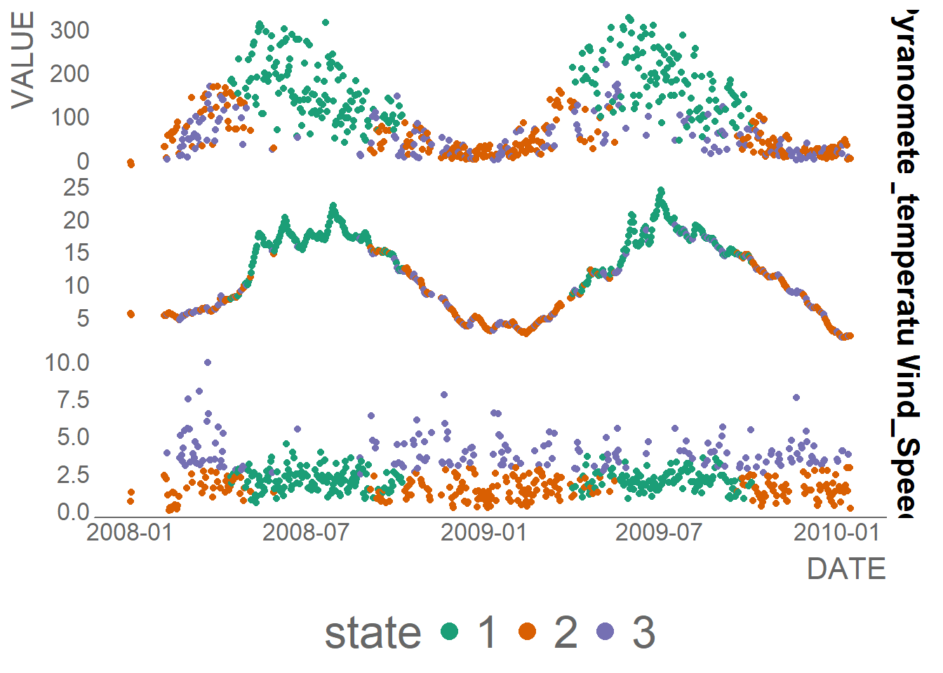
p1 = .Last.value
### 3D plotting of clusters
#| fig-cap: "A visual summary of the three clusters (e.g. cluster 3 represents high wind conditions)"
#| fig-alt: "A visual summary of the three clusters"


# 2D
plot(clusters)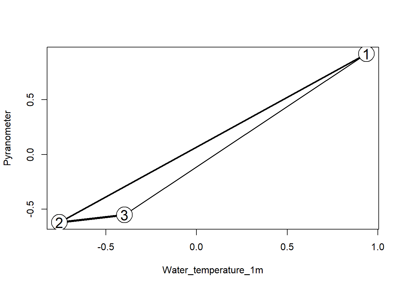
# 3Dmake cluster predictions
# not used, apply to hourly data directly

### predict hi-res data

### (1) no aggregation


newdata = Esthwaite_Buoy_HiRes |> rename(Water_temperature_1m=Temp1m,Pyranometer=SPFD,Wind_Speed=WindSpd)

newdata = pred_clusters(clusters, newdata)

# plot hourly state and weather data
ggplot(newdata |> dplyr::select(TIMESTAMP,Water_temperature_1m,Pyranometer,Wind_Speed,state)  |>
    pivot_longer(!c(TIMESTAMP, state), names_to = "FIELDNAME", values_to = "VALUE") |>
    mutate(state = as.factor(state))
) +
  geom_point(aes(x=TIMESTAMP,y=VALUE, color=state)) +
  facet_grid(rows = vars(FIELDNAME), scales = "free") +
  theme_gov() +
  scale_colour_discrete(palette = scales::pal_brewer(palette = "Dark2")) +
  guides(color = guide_legend(override.aes = list(size = 4)))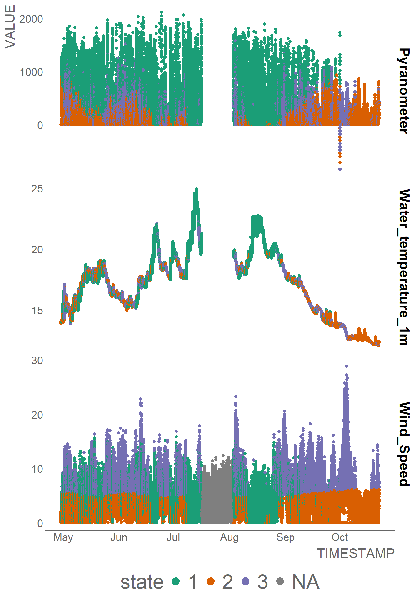
newdata  |>
      group_by(lubridate::date(TIMESTAMP )) |>
      summarise(across(where(is.numeric), mean, na.rm = TRUE)) |>
      dplyr::rename(DATE = 'lubridate::date(TIMESTAMP)')
# A tibble: 177 × 24
DATE RECORD AirTemp WindDir Wind_Speed CMP6 Pyranometer PonselTemp
<date> <dbl> <dbl> <dbl> <dbl> <dbl> <dbl> <dbl>
1 2025-04-29 32.7 11.5 81.0 1.36 0 0.0213 14.5
2 2025-04-30 434. 15.9 153. 2.23 280. 446. 15.5
3 2025-05-01 1154. 14.9 151. 4.95 283. 458. 16.3
4 2025-05-02 898. 12.4 101. 5.02 272. 442. 15.8
5 2025-05-03 655. 11.7 97.0 5.71 241. 380. 15.3
6 2025-05-04 412. 8.58 67.3 6.39 218. 342. 14.9
7 2025-05-05 1132. 9.02 96.9 4.81 233. 374. 14.4
8 2025-05-06 1852. 10.5 124. 2.96 272. 442. 15.0
9 2025-05-07 2572. 11.8 163. 3.27 276. 441. 15.5
10 2025-05-08 3292. 9.01 119. 2.88 166. 268. 15.4
# ℹ 167 more rows
# ℹ 16 more variables: PonselCond <dbl>, Temp_RH <dbl>, RH <dbl>,
# Water_temperature_1m <dbl>, Temp2m <dbl>, Temp3m <dbl>, Temp4m <dbl>,
# Temp5m <dbl>, Temp6m <dbl>, Temp7m <dbl>, Temp8m <dbl>, Temp9m <dbl>,
# Temp10m <dbl>, Temp11m <dbl>, Temp12m <dbl>, state <dbl>
Mode <- function(x) {
  ux <- unique(x)
  ux[which.max(tabulate(match(x, ux)))]
}

# Find state from previous 24 hour data (option 1: daily mode of states, option 2: do state tagging on daily mean data)
newdataDailyMode = newdata |> dplyr::select(TIMESTAMP,Water_temperature_1m,Pyranometer,Wind_Speed,state) |>
      group_by(lubridate::date(TIMESTAMP )) |>
      summarise(across(where(is.numeric), Mode)) |>
      dplyr::rename(DATE = 'lubridate::date(TIMESTAMP)') |>
      dplyr::mutate(state = lag(state))

newdataDailyMode
# A tibble: 177 × 5
DATE Water_temperature_1m Pyranometer Wind_Speed state
<date> <dbl> <dbl> <dbl> <int>
1 2025-04-29 14.0 0 0 NA
2 2025-04-30 14.0 0 0 2
3 2025-05-01 14.4 0 0 2
4 2025-05-02 15.0 0 0 2
5 2025-05-03 15.4 0 0 3
6 2025-05-04 15.4 0 8.69 2
7 2025-05-05 14.4 0 2.40 3
8 2025-05-06 14.4 0 0.000836 2
9 2025-05-07 15.0 0 0.745 2
10 2025-05-08 15.2 0 1.73 2
# ℹ 167 more rowsThis is the daily clustering rules we will apply. We apply daily state to high freq data and apply sampling rule by states:
- High Temp/ Low wind: every 10 min, starting from 0000
- Low Temp/ Low wind: every hour
- High wind: every 6 hours (0300,0900,1500,2100)
#| fig-cap: "Daily clustering results."
#| fig-alt: "Daily clustering results."

# Apply daily state to high freq data and apply sampling rule by states:
# 1. High Temp/ Low wind: every 10 min, starting from 0000
# 2. Low Temp/ Low wind: every hour
# 3. High wind: every 6 hours (0300,0900,1500,2100)

# Appply the rule then left join with high freq data

times = newdataDailyMode |> select(DATE,state) |> drop_na() |>
  rowwise() |>
  mutate(TIMESTAMP = case_when(
      state == 1 ~ list(seq(
      from = as_datetime(DATE),
      to   = as_datetime(DATE) + hours(23) + minutes(50),
      by   = "10 min"
    )),
      state == 2 ~ list(as_datetime(DATE) + hours(0:23)),
      state == 3 ~ list(as_datetime(DATE) + hours(c(3, 9, 15, 21))),

      .default = list(as_datetime(DATE) + hours(c(0)))
    )
) %>%
  unnest(TIMESTAMP) %>%
  ungroup()

# plot sampling state


ggplot(times |> mutate(y=state, state=as.factor(state))) +
  geom_point(aes(x=TIMESTAMP,y=y, color=state)) +
  theme_gov() +
  scale_colour_discrete(palette = scales::pal_brewer(palette = "Dark2")) +
  guides(color = guide_legend(override.aes = list(size = 4)))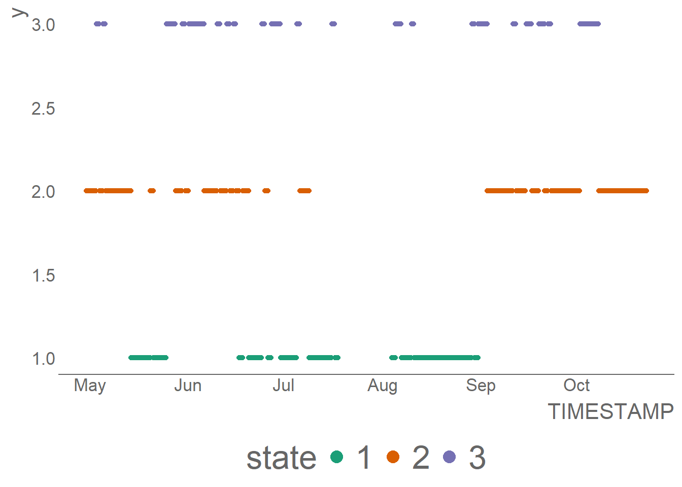
# left join, plot sampled weather data and their state
times |> mutate(y=state, state=as.factor(state)) |>
  left_join(newdata |> select(-state), by='TIMESTAMP') |>
  select(TIMESTAMP,Water_temperature_1m,Pyranometer,Wind_Speed,state)  |>
  pivot_longer(!c(TIMESTAMP, state), names_to = "FIELDNAME", values_to = "VALUE") |>
  ggplot() +
  geom_point(aes(x=TIMESTAMP,y=VALUE, color=state)) +
  facet_grid(rows = vars(FIELDNAME), scales = "free") +
  theme_gov() +
  scale_colour_discrete(palette = scales::pal_brewer(palette = "Dark2")) +
  guides(color = guide_legend(override.aes = list(size = 4)))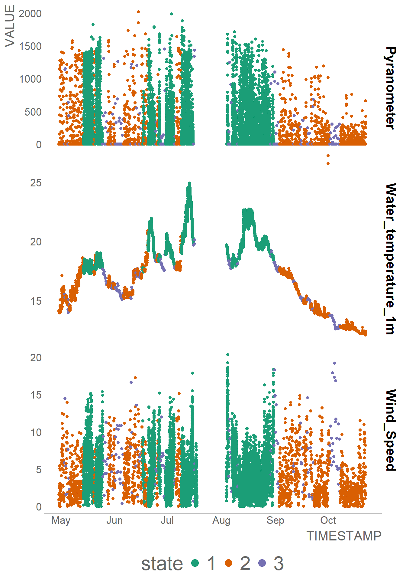
# left join, SUNA

rule_statetag <-times |> mutate(y=state, state=as.factor(state)) |>
  left_join(Esthwaite_Buoy_SUNA_Data , by='TIMESTAMP')

rule_statetag  |>
  ggplot() +
  geom_point(aes(x=TIMESTAMP,y=SUNA_Nitrate_mgL , color=state)) +
  theme_gov() +
  scale_colour_discrete(palette = scales::pal_brewer(palette = "Dark2")) +
  guides(color = guide_legend(override.aes = list(size = 4)))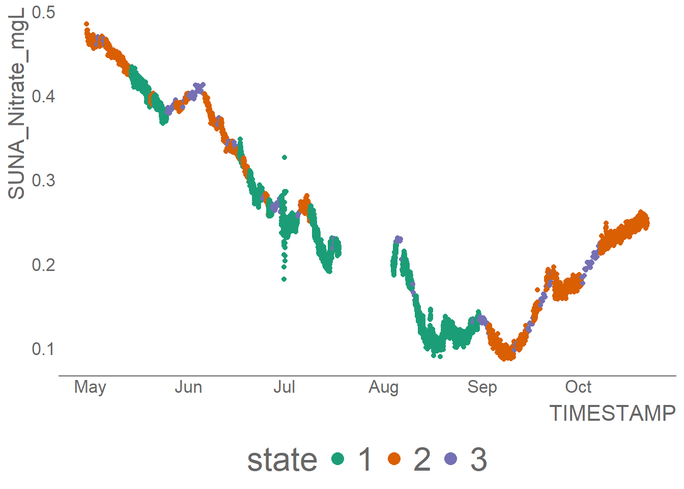
# metrics
a = diff(range(Esthwaite_Buoy_SUNA_Data$`SUNA_Nitrate_mgL`, na.rm = TRUE))
diff(range(rule_statetag$`SUNA_Nitrate_mgL`, na.rm = TRUE)) /a
[1] 0.9260465
b = median(Esthwaite_Buoy_SUNA_Data$`SUNA_Nitrate_mgL`, na.rm = TRUE)
(median(rule_statetag$`SUNA_Nitrate_mgL`, na.rm = TRUE) -b) /b
[1] -0.006919643