Fitting generalised additive models within jsdmstan

library(jsdmstan)

Background

The jsdmstan package supports the fitting of non-linear and random effects through using the generalised additive modelling (GAM) approach as represented within the mgcv R package (available on CRAN; Wood, 2011). See Wood (2025) for an overview of the GAM method. This means that the user can specify splines by using the formula argument to stan_jsdm() and including an s() call within that formula to specify the spline structure. This can be done either at the site-level (where multiple basis functions are supported) or at the species-level by fitting a factor-smooth to species. Examples of this in practice are shown below.

Site-specific splines

# 2 spline nfs testing ####
set.seed(2)
dat <- mgcv::gamSim(1,n=100,dist="normal",scale=2)
#> Gu & Wahba 4 term additive model
dat$flevels <- as.factor(rep(LETTERS[1:5],each=20))
dat$fvals <- rep(rnorm(5, sd = .5),each=20)

dat$y6 <- dat$f2 + dat$fvals + rnorm(100, sd=.5)
dat$y7 <- dat$f2 + dat$fvals + rnorm(100, sd=.5)
dat$y8 <- dat$f2 + dat$fvals + rnorm(100, sd=.5)
dat$y9 <- dat$f2 + dat$fvals + rnorm(100, sd=.5)

Y <- dat[,c("y6","y7","y8","y9")]

Model fit, specifying priors for beta (representing the intercept only, in this case) based upon the data:

nfs_fit <- stan_jsdm(~s(x2) + s(flevels, bs = "re"), data = dat,
                     Y = Y, family ="gaussian", method = "mglmm",
                     prior = jsdm_prior(betas = "normal(3,1)"),
                     iter = 1000)
#> 
#> SAMPLING FOR MODEL 'anon_model' NOW (CHAIN 1).
#> Chain 1: 
#> Chain 1: Gradient evaluation took 0.000162 seconds
#> Chain 1: 1000 transitions using 10 leapfrog steps per transition would take 1.62 seconds.
#> Chain 1: Adjust your expectations accordingly!
#> Chain 1: 
#> Chain 1: 
#> Chain 1: Iteration:   1 / 1000 [  0%]  (Warmup)
#> Chain 1: Iteration: 100 / 1000 [ 10%]  (Warmup)
#> Chain 1: Iteration: 200 / 1000 [ 20%]  (Warmup)
#> Chain 1: Iteration: 300 / 1000 [ 30%]  (Warmup)
#> Chain 1: Iteration: 400 / 1000 [ 40%]  (Warmup)
#> Chain 1: Iteration: 500 / 1000 [ 50%]  (Warmup)
#> Chain 1: Iteration: 501 / 1000 [ 50%]  (Sampling)
#> Chain 1: Iteration: 600 / 1000 [ 60%]  (Sampling)
#> Chain 1: Iteration: 700 / 1000 [ 70%]  (Sampling)
#> Chain 1: Iteration: 800 / 1000 [ 80%]  (Sampling)
#> Chain 1: Iteration: 900 / 1000 [ 90%]  (Sampling)
#> Chain 1: Iteration: 1000 / 1000 [100%]  (Sampling)
#> Chain 1: 
#> Chain 1:  Elapsed Time: 9.385 seconds (Warm-up)
#> Chain 1:                9.929 seconds (Sampling)
#> Chain 1:                19.314 seconds (Total)
#> Chain 1: 
#> 
#> SAMPLING FOR MODEL 'anon_model' NOW (CHAIN 2).
#> Chain 2: 
#> Chain 2: Gradient evaluation took 9.9e-05 seconds
#> Chain 2: 1000 transitions using 10 leapfrog steps per transition would take 0.99 seconds.
#> Chain 2: Adjust your expectations accordingly!
#> Chain 2: 
#> Chain 2: 
#> Chain 2: Iteration:   1 / 1000 [  0%]  (Warmup)
#> Chain 2: Iteration: 100 / 1000 [ 10%]  (Warmup)
#> Chain 2: Iteration: 200 / 1000 [ 20%]  (Warmup)
#> Chain 2: Iteration: 300 / 1000 [ 30%]  (Warmup)
#> Chain 2: Iteration: 400 / 1000 [ 40%]  (Warmup)
#> Chain 2: Iteration: 500 / 1000 [ 50%]  (Warmup)
#> Chain 2: Iteration: 501 / 1000 [ 50%]  (Sampling)
#> Chain 2: Iteration: 600 / 1000 [ 60%]  (Sampling)
#> Chain 2: Iteration: 700 / 1000 [ 70%]  (Sampling)
#> Chain 2: Iteration: 800 / 1000 [ 80%]  (Sampling)
#> Chain 2: Iteration: 900 / 1000 [ 90%]  (Sampling)
#> Chain 2: Iteration: 1000 / 1000 [100%]  (Sampling)
#> Chain 2: 
#> Chain 2:  Elapsed Time: 11.804 seconds (Warm-up)
#> Chain 2:                10.249 seconds (Sampling)
#> Chain 2:                22.053 seconds (Total)
#> Chain 2: 
#> 
#> SAMPLING FOR MODEL 'anon_model' NOW (CHAIN 3).
#> Chain 3: 
#> Chain 3: Gradient evaluation took 9e-05 seconds
#> Chain 3: 1000 transitions using 10 leapfrog steps per transition would take 0.9 seconds.
#> Chain 3: Adjust your expectations accordingly!
#> Chain 3: 
#> Chain 3: 
#> Chain 3: Iteration:   1 / 1000 [  0%]  (Warmup)
#> Chain 3: Iteration: 100 / 1000 [ 10%]  (Warmup)
#> Chain 3: Iteration: 200 / 1000 [ 20%]  (Warmup)
#> Chain 3: Iteration: 300 / 1000 [ 30%]  (Warmup)
#> Chain 3: Iteration: 400 / 1000 [ 40%]  (Warmup)
#> Chain 3: Iteration: 500 / 1000 [ 50%]  (Warmup)
#> Chain 3: Iteration: 501 / 1000 [ 50%]  (Sampling)
#> Chain 3: Iteration: 600 / 1000 [ 60%]  (Sampling)
#> Chain 3: Iteration: 700 / 1000 [ 70%]  (Sampling)
#> Chain 3: Iteration: 800 / 1000 [ 80%]  (Sampling)
#> Chain 3: Iteration: 900 / 1000 [ 90%]  (Sampling)
#> Chain 3: Iteration: 1000 / 1000 [100%]  (Sampling)
#> Chain 3: 
#> Chain 3:  Elapsed Time: 10.798 seconds (Warm-up)
#> Chain 3:                10.284 seconds (Sampling)
#> Chain 3:                21.082 seconds (Total)
#> Chain 3: 
#> 
#> SAMPLING FOR MODEL 'anon_model' NOW (CHAIN 4).
#> Chain 4: 
#> Chain 4: Gradient evaluation took 9.1e-05 seconds
#> Chain 4: 1000 transitions using 10 leapfrog steps per transition would take 0.91 seconds.
#> Chain 4: Adjust your expectations accordingly!
#> Chain 4: 
#> Chain 4: 
#> Chain 4: Iteration:   1 / 1000 [  0%]  (Warmup)
#> Chain 4: Iteration: 100 / 1000 [ 10%]  (Warmup)
#> Chain 4: Iteration: 200 / 1000 [ 20%]  (Warmup)
#> Chain 4: Iteration: 300 / 1000 [ 30%]  (Warmup)
#> Chain 4: Iteration: 400 / 1000 [ 40%]  (Warmup)
#> Chain 4: Iteration: 500 / 1000 [ 50%]  (Warmup)
#> Chain 4: Iteration: 501 / 1000 [ 50%]  (Sampling)
#> Chain 4: Iteration: 600 / 1000 [ 60%]  (Sampling)
#> Chain 4: Iteration: 700 / 1000 [ 70%]  (Sampling)
#> Chain 4: Iteration: 800 / 1000 [ 80%]  (Sampling)
#> Chain 4: Iteration: 900 / 1000 [ 90%]  (Sampling)
#> Chain 4: Iteration: 1000 / 1000 [100%]  (Sampling)
#> Chain 4: 
#> Chain 4:  Elapsed Time: 11.595 seconds (Warm-up)
#> Chain 4:                10.269 seconds (Sampling)
#> Chain 4:                21.864 seconds (Total)
#> Chain 4:
#> Warning: Bulk Effective Samples Size (ESS) is too low, indicating posterior means and medians may be unreliable.
#> Running the chains for more iterations may help. See
#> https://mc-stan.org/misc/warnings.html#bulk-ess
#> Warning: Tail Effective Samples Size (ESS) is too low, indicating posterior variances and tail quantiles may be unreliable.
#> Running the chains for more iterations may help. See
#> https://mc-stan.org/misc/warnings.html#tail-ess

There’s a couple of warnings on ESS, so we’ll check to see what is going on by printing the model object to the console:

nfs_fit
#> Family: gaussian 
#>  With parameters: sigma 
#> Model type: mglmm
#>   Number of species: 4
#>   Number of sites: 100
#>   Number of predictors: 0
#> 
#> Model run on 4 chains with 1000 iterations per chain (500 warmup).
#> 
#> Parameters with Rhat > 1.01, or Neff/N < 0.05:
#>          mean     sd      15%      85% Rhat Bulk.ESS Tail.ESS
#> lp__ -134.182 23.739 -158.558 -110.844 1.01      285      384

There are several parameters with ESS < 500, but the ESS is always over 400 which should be fine for our purposes. Now we can look at model recovery of the data, using the standard jsdmstan functions. We’ll just take a look to see if the model recovers the individual species distributions:

multi_pp_check(nfs_fit)
#> Using 10 posterior draws for ppc plot type 'ppc_dens_overlay' by default.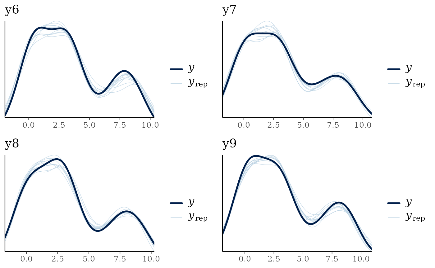

The model seems to recover the data well. We can also plot out the smooth effects using the smoothplot() function. This returns a list of ggplot2 objects including plots for each smooth fitted. For smooths such as the default thin-plate regression spline or e.g. a cyclic cubic regression spline this will take the form of a series of lines representing different draws from the model. For random effect splines this takes the form of a jittered point plot of the random effect values plotted against the random effect categories. The number of draws can be varied, and a summary line added to the line plots if required.

smoothplot(nfs_fit)
#> [[1]]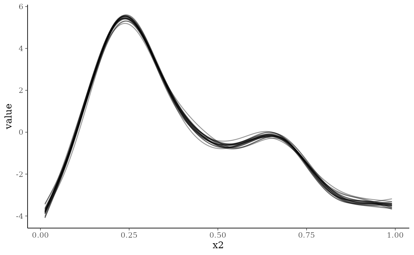

#> 
#> [[2]]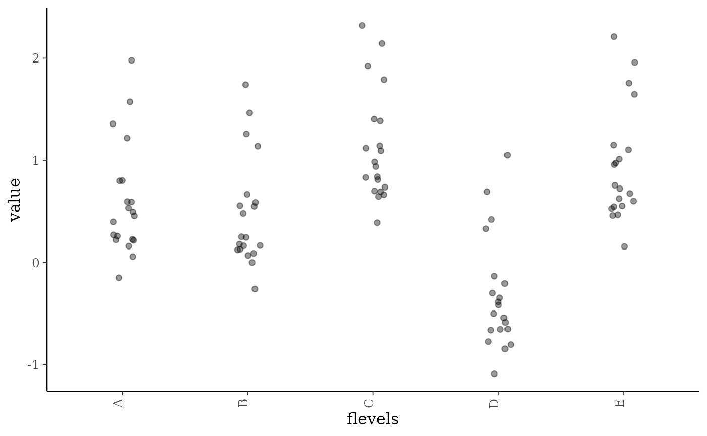

To demonstrate some of the smoothplot options, here we’ll plot the average smooth from 1000 draws for the first smooth (not the random effect):

smoothplot(nfs_fit, summarise = mean, ndraws = 1000, 
           select_smooths = list(site = 1))
#> [[1]]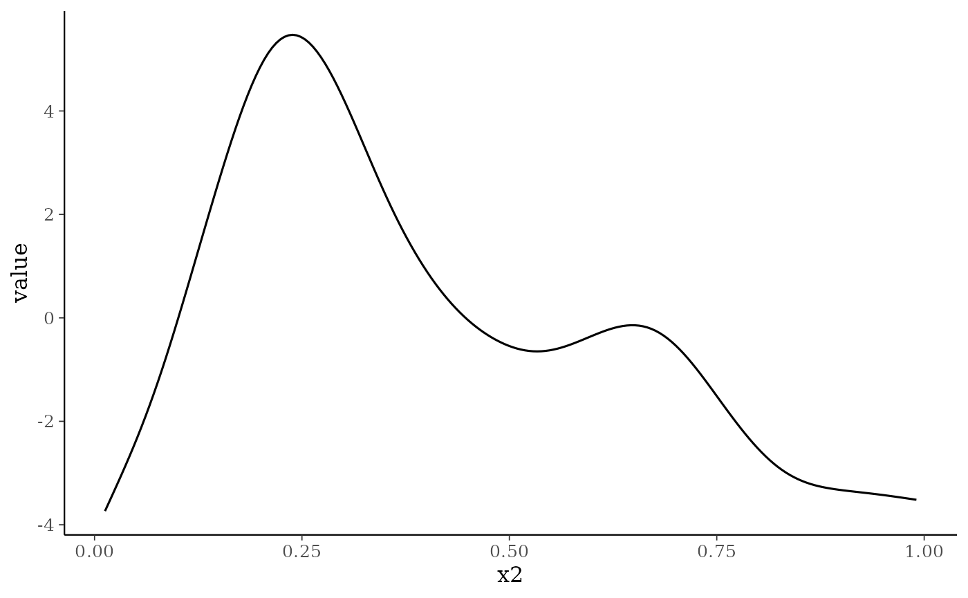

Species- and site-specific factor smooths

Simulate data, based upon the factor-smooth example in the mgcv::gam() documentation:

set.seed(0)
## simulate data...
f1 <- function(x,a=2,b=-1) exp(a * x)+b
n <- 500;nf <- 6
fac <- as.factor(rep(LETTERS[1:nf],each=50))
x1 <- rep(runif(50),nf)
a <- rnorm(nf)*.2 + 2;b <- rnorm(nf)*.5
f <- f1(x1,a[fac],b[fac])
fac <- factor(fac)
y <- f + rnorm(n)
#> Warning in f + rnorm(n): longer object length is not a multiple of shorter
#> object length

So response depends on a smooth of x1 for each level of fac, which we now convert the data into wide format:

df <- data.frame(x1 = x1[1:50])
Y <- matrix(y, nrow = 50)
colnames(Y) <- LETTERS[1:10]

We fit the model by specifying species as the factor within a factor-smooth model. Species doesn’t need to be in the original dataframe (and obviously cannot be!) as jsdmstan recognises what is going on and sorts it all out under the hood. Note that if species is a column name in the original dataframe it will be ignored and instead the model fit to vary across the columns of Y. Specifying any other column name as the factor within the factor-smooth means that jsdmstan will fit a site-specific factor instead.

fs1_fit <- stan_jsdm(~s(x1, species, bs = "fs"), data = df, Y = Y,
                     family = "gaussian", method = "mglmm", iter = 1000)
#> 
#> SAMPLING FOR MODEL 'anon_model' NOW (CHAIN 1).
#> Chain 1: 
#> Chain 1: Gradient evaluation took 0.001557 seconds
#> Chain 1: 1000 transitions using 10 leapfrog steps per transition would take 15.57 seconds.
#> Chain 1: Adjust your expectations accordingly!
#> Chain 1: 
#> Chain 1: 
#> Chain 1: Iteration:   1 / 1000 [  0%]  (Warmup)
#> Chain 1: Iteration: 100 / 1000 [ 10%]  (Warmup)
#> Chain 1: Iteration: 200 / 1000 [ 20%]  (Warmup)
#> Chain 1: Iteration: 300 / 1000 [ 30%]  (Warmup)
#> Chain 1: Iteration: 400 / 1000 [ 40%]  (Warmup)
#> Chain 1: Iteration: 500 / 1000 [ 50%]  (Warmup)
#> Chain 1: Iteration: 501 / 1000 [ 50%]  (Sampling)
#> Chain 1: Iteration: 600 / 1000 [ 60%]  (Sampling)
#> Chain 1: Iteration: 700 / 1000 [ 70%]  (Sampling)
#> Chain 1: Iteration: 800 / 1000 [ 80%]  (Sampling)
#> Chain 1: Iteration: 900 / 1000 [ 90%]  (Sampling)
#> Chain 1: Iteration: 1000 / 1000 [100%]  (Sampling)
#> Chain 1: 
#> Chain 1:  Elapsed Time: 67.97 seconds (Warm-up)
#> Chain 1:                42.279 seconds (Sampling)
#> Chain 1:                110.249 seconds (Total)
#> Chain 1: 
#> 
#> SAMPLING FOR MODEL 'anon_model' NOW (CHAIN 2).
#> Chain 2: 
#> Chain 2: Gradient evaluation took 0.001345 seconds
#> Chain 2: 1000 transitions using 10 leapfrog steps per transition would take 13.45 seconds.
#> Chain 2: Adjust your expectations accordingly!
#> Chain 2: 
#> Chain 2: 
#> Chain 2: Iteration:   1 / 1000 [  0%]  (Warmup)
#> Chain 2: Iteration: 100 / 1000 [ 10%]  (Warmup)
#> Chain 2: Iteration: 200 / 1000 [ 20%]  (Warmup)
#> Chain 2: Iteration: 300 / 1000 [ 30%]  (Warmup)
#> Chain 2: Iteration: 400 / 1000 [ 40%]  (Warmup)
#> Chain 2: Iteration: 500 / 1000 [ 50%]  (Warmup)
#> Chain 2: Iteration: 501 / 1000 [ 50%]  (Sampling)
#> Chain 2: Iteration: 600 / 1000 [ 60%]  (Sampling)
#> Chain 2: Iteration: 700 / 1000 [ 70%]  (Sampling)
#> Chain 2: Iteration: 800 / 1000 [ 80%]  (Sampling)
#> Chain 2: Iteration: 900 / 1000 [ 90%]  (Sampling)
#> Chain 2: Iteration: 1000 / 1000 [100%]  (Sampling)
#> Chain 2: 
#> Chain 2:  Elapsed Time: 64.562 seconds (Warm-up)
#> Chain 2:                42.226 seconds (Sampling)
#> Chain 2:                106.788 seconds (Total)
#> Chain 2: 
#> 
#> SAMPLING FOR MODEL 'anon_model' NOW (CHAIN 3).
#> Chain 3: 
#> Chain 3: Gradient evaluation took 0.001333 seconds
#> Chain 3: 1000 transitions using 10 leapfrog steps per transition would take 13.33 seconds.
#> Chain 3: Adjust your expectations accordingly!
#> Chain 3: 
#> Chain 3: 
#> Chain 3: Iteration:   1 / 1000 [  0%]  (Warmup)
#> Chain 3: Iteration: 100 / 1000 [ 10%]  (Warmup)
#> Chain 3: Iteration: 200 / 1000 [ 20%]  (Warmup)
#> Chain 3: Iteration: 300 / 1000 [ 30%]  (Warmup)
#> Chain 3: Iteration: 400 / 1000 [ 40%]  (Warmup)
#> Chain 3: Iteration: 500 / 1000 [ 50%]  (Warmup)
#> Chain 3: Iteration: 501 / 1000 [ 50%]  (Sampling)
#> Chain 3: Iteration: 600 / 1000 [ 60%]  (Sampling)
#> Chain 3: Iteration: 700 / 1000 [ 70%]  (Sampling)
#> Chain 3: Iteration: 800 / 1000 [ 80%]  (Sampling)
#> Chain 3: Iteration: 900 / 1000 [ 90%]  (Sampling)
#> Chain 3: Iteration: 1000 / 1000 [100%]  (Sampling)
#> Chain 3: 
#> Chain 3:  Elapsed Time: 64.475 seconds (Warm-up)
#> Chain 3:                42.304 seconds (Sampling)
#> Chain 3:                106.779 seconds (Total)
#> Chain 3: 
#> 
#> SAMPLING FOR MODEL 'anon_model' NOW (CHAIN 4).
#> Chain 4: 
#> Chain 4: Gradient evaluation took 0.001315 seconds
#> Chain 4: 1000 transitions using 10 leapfrog steps per transition would take 13.15 seconds.
#> Chain 4: Adjust your expectations accordingly!
#> Chain 4: 
#> Chain 4: 
#> Chain 4: Iteration:   1 / 1000 [  0%]  (Warmup)
#> Chain 4: Iteration: 100 / 1000 [ 10%]  (Warmup)
#> Chain 4: Iteration: 200 / 1000 [ 20%]  (Warmup)
#> Chain 4: Iteration: 300 / 1000 [ 30%]  (Warmup)
#> Chain 4: Iteration: 400 / 1000 [ 40%]  (Warmup)
#> Chain 4: Iteration: 500 / 1000 [ 50%]  (Warmup)
#> Chain 4: Iteration: 501 / 1000 [ 50%]  (Sampling)
#> Chain 4: Iteration: 600 / 1000 [ 60%]  (Sampling)
#> Chain 4: Iteration: 700 / 1000 [ 70%]  (Sampling)
#> Chain 4: Iteration: 800 / 1000 [ 80%]  (Sampling)
#> Chain 4: Iteration: 900 / 1000 [ 90%]  (Sampling)
#> Chain 4: Iteration: 1000 / 1000 [100%]  (Sampling)
#> Chain 4: 
#> Chain 4:  Elapsed Time: 71.699 seconds (Warm-up)
#> Chain 4:                42.253 seconds (Sampling)
#> Chain 4:                113.952 seconds (Total)
#> Chain 4:
#> Warning: Bulk Effective Samples Size (ESS) is too low, indicating posterior means and medians may be unreliable.
#> Running the chains for more iterations may help. See
#> https://mc-stan.org/misc/warnings.html#bulk-ess
#> Warning: Tail Effective Samples Size (ESS) is too low, indicating posterior variances and tail quantiles may be unreliable.
#> Running the chains for more iterations may help. See
#> https://mc-stan.org/misc/warnings.html#tail-ess

There is one warning about effective sample size, so we can print the model object to see which parameters had low ESS:

fs1_fit
#> Family: gaussian 
#>  With parameters: sigma 
#> Model type: mglmm
#>   Number of species: 10
#>   Number of sites: 50
#>   Number of predictors: 0
#> 
#> Model run on 4 chains with 1000 iterations per chain (500 warmup).
#> 
#> No parameters with Rhat > 1.01 or Neff/N < 0.05

An effective sample size of over 200 seems like it should be fine for our purposes here, although you may want to run for more iterations if this was to be used for more than instructional purposes.

The recovery of the data can be evaluated by using functions such as pp_check() or multi_pp_check(). This model seems to recover the data well.

multi_pp_check(fs1_fit)
#> Using 10 posterior draws for ppc plot type 'ppc_dens_overlay' by default.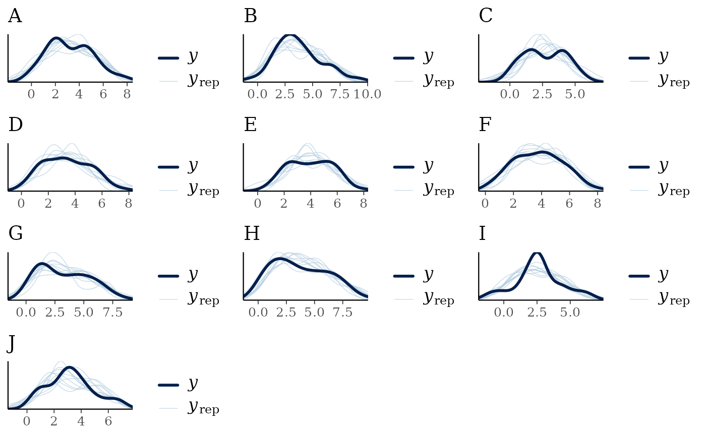

For factor smooths the smoothplot() function returns a ggplot2 object facetted by the factor (here species, but within the site-specific factor smooths this could be any factor specified by the user).

smoothplot(fs1_fit)
#> [[1]]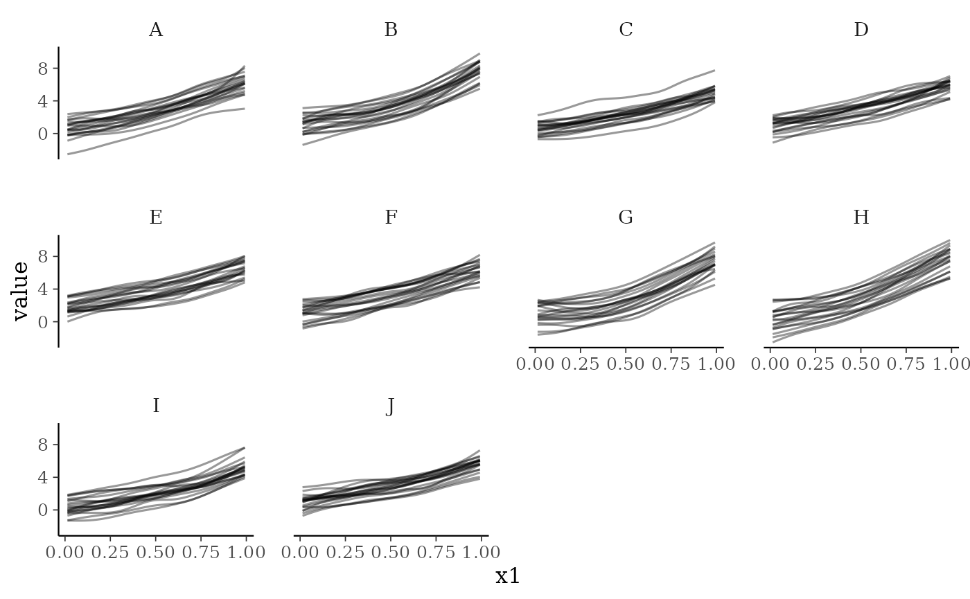

Comments

A mix of site-specific and species-specific smooths can also be fit, as can many different types of smooth basis functions. Not all types of smooth basis functions have been tested yet, and it is entirely possible that some smooths will be fit that cannot be plotted or predicted correctly from - please raise an issue at https://github.com/NERC-CEH/jsdmstan/issues if you run into any problems or have a type of smooth that you’d like to be able to fit but cannot.

References

Wood, S.N. (2011) Fast stable restricted maximum likelihood and marginal likelihood estimation of semiparametric generalized linear models. Journal of the Royal Statistical Society (B) 73(1):3-36

Wood, S.N. (2025) Generalized Additive Models. Annual Review Statistics and Its Application. 12:497-526. https://doi.org/10.1146/annurev-statistics-112723-034249