Fine-Tuning a Geospatial Foundation Model for UK Crop Classification

Prithvi-EO-2.0 UK Crop Map Classification¶

Challenge and Methodological Approach Summary¶

Currently, UKCEH Land Cover® plus: Crops is updated using supervised learning methods that depend heavily on high-quality labelled training data. Much of this data is inherited from previous versions, which works well for existing classes. However, when new analytical needs arise, such as adding extra classes, there is a significant time and resource cost involved in generating sufficient new labelled data. Prithvi-EO-2.0 is a multi-temporal geospatial foundation model that is trained on millions of global time series samples from NASA’s Harmonized Landsat and Sentinel-2 data archive.

This notebook demonstrates how to fine-tune Prithvi-2.0-EO using TerraTorch for a multi-temporal crop classification task. It covers setting up the environment, preparing the data using a custom CropDataModule, configuring and training a semantic segmentation model, and evaluating its performance.

Core Concepts & Frameworks¶

Earth Observation (EO): The field of collecting and analyzing information about Earth’s physical, chemical, and biological systems through remote sensing techniques, often using satellite imagery.
Foundation Model: A large, pre-trained deep learning model designed to perform a wide range of tasks. It learns general features from vast amounts of data and can be adapted (fine-tuned) for specific downstream applications.
Prithvi foundation model: A specific foundation model developed by IBM for Earth observation (EO) data. It learns features from satellite imagery and is designed to be fine-tuned for various geospatial tasks.
TerraTorch: An open-source Python library built on PyTorch that provides tools and functionalities specifically for working with geospatial and Earth observation data, facilitating the development and application of deep learning models, including foundation models like Prithvi.

Data & Preprocessing¶

Multi-temporal Classification: A machine learning task that involves classifying land cover or objects by analyzing a sequence of satellite images taken over different time points (i.e., multiple timestamps). This helps to capture changes and temporal patterns.
DataModule (PyTorch Lightning): A high-level abstraction in PyTorch Lightning that encapsulates all data-related logic for a deep learning project, including data loading, preprocessing, augmentation, and splitting into training, validation, and test sets.
CropDataModule: A specialized DataModule implementation within TerraTorch designed to handle the specific multi-temporal crop classification dataset used in this notebook.
batch_size: The number of samples processed together in one forward/backward pass during training.
num_workers: The number of subprocesses used for data loading to speed up the data fetching process.
data_root: The base directory path where the dataset files are stored.
Transformations: Operations applied to input data (e.g., images) for augmentation (to increase data variability) or preprocessing (e.g., normalization, resizing) before feeding them into the model.
Spectral Bands: Different ranges of electromagnetic radiation (wavelengths) captured by sensors (e.g., satellite imagery). Common bands include Blue, Green, Red, Near-Infrared (NIR), and Short-Wave Infrared (SWIR).

Model Training & Evaluation¶

Semantic Segmentation: A computer vision task that involves classifying every pixel in an image into a predefined category. In this context, it means classifying each pixel in a satellite image as a particular crop type.
Fine-tuning: The process of taking a pre-trained model (like Prithvi) and continuing its training on a new, specific dataset for a related task. This often requires less data and computational resources than training from scratch.
Trainer (PyTorch Lightning): The central object in PyTorch Lightning that orchestrates the entire training loop, including optimization, logging, checkpointing, and evaluation.
ModelCheckpoint: A PyTorch Lightning callback that automatically saves the model’s weights during training, typically saving the best-performing model based on a monitored metric.
SemanticSegmentationTask: A specific task implementation within TerraTorch designed for semantic segmentation problems, providing an interface to define model architecture, loss, and metrics.
accelerator: Specifies the type of hardware used for training (e.g., ‘gpu’, ‘cpu’, ‘tpu’).
precision: Defines the numerical precision used for computations during training (e.g., 16-mixed for mixed-precision training, which can speed up training and reduce memory usage).
max_epochs: The maximum number of times the entire training dataset will be passed through the model during training.
backbone: The feature extraction part of a deep learning model, typically a pre-trained convolutional neural network (CNN) or a Vision Transformer (ViT), which learns hierarchical representations of the input data.
decoder: In semantic segmentation models, the decoder takes the features extracted by the backbone and upsamples them to reconstruct an output image (segmentation mask) at the original input resolution.
head: The final layer(s) of a deep learning model that produce the task-specific output (e.g., class probabilities for classification, pixel-wise predictions for segmentation).
loss function (loss): A mathematical function that quantifies the difference between the model’s predictions and the true labels. The goal of training is to minimize this function.
Learning Rate (lr): A hyperparameter that determines the step size at which an optimizer adjusts the model’s weights during training.
Optimizer: An algorithm (e.g., Adam, SGD) used to adjust the weights and biases of a neural network to minimize the loss function.
freeze_backbone, freeze_decoder: Techniques used during fine-tuning where the weights of specific parts of the model (e.g., the backbone or decoder) are kept fixed and are not updated during the training process, often to preserve pre-trained knowledge.
TensorBoard: A web-based visualization tool provided by TensorFlow (and compatible with PyTorch Lightning) that allows tracking training metrics (loss, accuracy), visualizing model graphs, and analyzing embeddings.
Checkpoint: A saved state of a deep learning model at a particular point during training, including its architecture, weights, optimizer state, and other metadata. This allows for resuming training or loading the best model for inference.

Running the Notebook

Data Access

Statistical Concepts

Generalisability

This notebook can currently be run in Google Colab by clicking .

To run this notebook, you must first download the required module files from the GitHub Repository. Access to a Google Colab subscription may also be beneficial, as training the model can be computationally intensive. Lastly, you will need a dataset. The dataset used in this notebook was derived from Sentinel-2 and UKCEH Land Cover® plus: Crops. UKCEH Land Cover® plus: Crops is available under licence for internal business use, for academic research/education and for use in innovation and value added reselling. For Academic Research/Education only, UKCEH Land Cover® plus: Crops datasets are available for free via EDINA, specifically the Environment section.

Introduction¶

This project aims to develop and validate a data efficient crop classification pipeline that leverages the pretrained spatial-temporal representations of Prithvi-EO-2.0. Through either fine-tuning or acting as a front-end feature extractor for an existing Random Forest classifier, the outcome of this project could assist in reducing ground truth data dependencies, eliminating manual feature engineering, and minimising spatial classification noise.

The UKCEH Land Cover® plus: Crops dataset is important for policy makers, regulatory agencies and scientists. It’s used in hydrological modelling, crop science, and other environmental science purposes. Currently, UKCEH Land Cover® plus: Crops is updated using supervised learning methods that depend heavily on high-quality labelled training data. Much of this data is inherited from previous versions, which works well for existing classes. However, when new analytical needs arise, such as adding classes, there is a significant time and resource cost involved in generating sufficient new labelled data. Prithvi-EO-2.0 is a geospatial foundation model that is trained on millions of global time series samples from NASA’s Harmonized Landsat and Sentinel-2 data archive. In this project we explored the potential use and performance of Prithvi-EO-2.0 for UK crop classification.

The dataset we used included ~900 raster GeoTIFF input chips (images and labels). Image chips were extracted from Sentinel-2. Each image chip contains 18 bands including 6 spectral bands for three time-steps stacked together. Label chips are from UKCEH Land Cover ® Plus: Crops classified into 16 classes containing one band with the target classes for each pixel. The ~900 chips were randomly split into training (60%), validation (20%), and testing (20%) subsets. The preprocessing workflow was done in QGIS, and the model analysis was performed using Python in Google Colab. Training was optimized with AdamW, at a learning rate of 0.0001 for 50 epochs, and a frozen backbone. Data augmentations such as random rotations were applied to minimise spatial biases. This initial proof of concept project demonstrates that Prithvi-2.0-EO can learn useful representations for UK crop classification from a relatively small, labelled dataset. After training, Prithvi-2.0-EO achieved 66.2% overall accuracy and 53.9% mean IoU across 16 classes, with a macro F1 score of 66.9%.

Importing Libraries and Loading Data¶

Setup¶

In colab: Go to “Runtime” -> “Change runtime type” -> Select “T4 GPU”

First we need to install the terratorch library along with gdown (for downloading files from Google Drive) and tensorboard (for visualizing training metrics). It also ensures specific compatible versions of torch, torchvision, and albumentations are installed or uninstalled to meet terratorch’s dependencies.

!pip install terratorch==1.2.1 # The fine-tuning toolkit needed
!pip install gdown tensorboard # Tensorboard is a model visualisation toolkit which offers graphs, histograms etc
!pip install -U jupyter ipywidgets # Jupyter Widgets allow you to add interactive controls like sliders, buttons, and text boxes to your notebook
!pip install rasterio # Rasterio allows users to handle geospatial raster datasets
!pip install albumentations # Albumentations is used for image augmentation, it can improve model generalization by creating varied training samples from existing images by rotating them etc

After installation we must import all the necessary Python libraries that will be used throughout the notebook. This includes standard libraries like os and sys, deep learning frameworks like torch and lightning.pytorch (aliased as pl).

Dataset and Module Imports¶

Now we need to mount your Google Drive to the notebook. Ensure that your notebook is in the same folder as the modules.

drive.mount("/content/drive")

os.chdir("/content/drive/MyDrive/datamodules") # The folder containing the modules, python files with prewritten functions and classes

DATA_ROOT = "/content/drive/MyDrive/dataset" # The folder containing two folders named "images" and "masks"

Datamodule Loading¶

Next we will list the contents of the directory. It helps to verify that the modules are in their expected file path.

!ls datamodules # Expected output: crop_datamodule.py  __init__.py  __pycache__

crop_datamodule.py  __init__.py  __pycache__

Following this, we will look at the dimensions of our chips. The output of the cell below should show that each chip has a shape of (bands, height, width). In this case, each chip is 224x224 pixels. The first number is the amount of bacthes (2), followed by the dimension (18) corresponding to the number of bands (6 bands * 3 time steps = 18 bands).

sys.path.insert(0, '/content/drive/MyDrive/datamodules')


from datamodules.crop_datamodule import CropDataModule # Datamodule classes and functions
from transforms.augmentations import train_transform

dm = CropDataModule(
    data_root=DATA_ROOT,
    batch_size=2,
    train_transform=train_transform,
    num_workers=2
)
dm.setup()

batch = next(iter(dm.train_dataloader()))
print("Image Batch Shape:", batch["image"].shape) # Expected output: torch.Size([2, 6, 3, H, W])
print("Mask Batch Shape:", batch["mask"].shape)   # Expected output: torch.Size([2, H, W])

Image Batch Shape: torch.Size([2, 6, 3, 224, 224])
Mask Batch Shape: torch.Size([2, 224, 224])

Fine-tuning¶

Model creation¶

The SemanticSegmentationTask uses the Prithvi backbone (specifically prithvi_eo_v2_300_tl) and defines the decoder, head, loss function, learning rate, and whether to freeze parts of the model for efficient fine-tuning.

model = SemanticSegmentationTask(
    model_factory="EncoderDecoderFactory",

    model_args={
        "backbone": "prithvi_eo_v2_300_tl",
        "backbone_pretrained": True,
        "backbone_num_frames": 3,
        "backbone_bands": [
            "BLUE",
            "GREEN",
            "RED",
            "NIR_NARROW",
            "SWIR_1",
            "SWIR_2"
        ],
        "backbone_coords_encoding": [],
        "necks": [
            {
                "name": "SelectIndices",
                "indices": [5, 11, 17, 23]
            },
            {
                "name": "ReshapeTokensToImage",
                "effective_time_dim": 3
            },
            {
                "name": "LearnedInterpolateToPyramidal"
            }
        ],
        "decoder": "UNetDecoder",
        "decoder_channels": [
            512,
            256,
            128,
            64
        ],
        "head_dropout": 0.1,
        "num_classes": 16
    },

    optimizer="AdamW",
    lr=1e-4,
    loss="ce",

    ignore_index=-1,

    freeze_backbone=True,

    plot_on_val=False
)

Checkpoints¶

The checkpoint and trainer cell sets up the PyTorch Lightning Trainer. The Trainer is configured with settings like accelerator, number of devices, precision, logging, and callbacks (e.g., ModelCheckpoint to save the best model)

checkpoint_callback = pl.callbacks.ModelCheckpoint(
    dirpath="checkpoints",
    filename="best-{epoch:02d}",
    save_top_k=1
)

trainer = pl.Trainer(
    accelerator="auto",
    devices=1,
    precision="bf16-mixed",
    max_epochs=50,
    callbacks=[checkpoint_callback]
)

Trainer¶

This cell initiates the training (fine-tuning) process. It calls the fit method on the trainer object, passing the model and the datamodule. The model will be trained for the specified number of epochs, with progress and metrics logged to TensorBoard and checkpoints saved based on the ModelCheckpoint callback.

trainer.fit(
    model,
    datamodule=dm
)

Validation Metrics and Plots¶

This cell loads the tensorboard extension for Jupyter notebooks and then starts a TensorBoard server. TensorBoard is a visualization tool that allows you to track and visualize metrics like loss and accuracy during the model training process, with logs stored in the output directory.

%load_ext tensorboard
%tensorboard --logdir lightning_logs
#%reload_ext tensorboard # Remove comment if you need to reload

Test Metrics¶

This cell defines a variable best_ckpt_path that stores the file path to the best model checkpoint saved during the training process. This checkpoint typically represents the model with the highest validation performance.

best_ckpt_path = trainer.checkpoint_callback.best_model_path

print(best_ckpt_path)

This cell evaluates the fine-tuned model on the unseen test dataset. It uses the test method of the trainer, loading the best model identified by best_ckpt_path. This provides an unbiased measure of the model’s generalization performance.

trainer.test(
    model,
    datamodule=dm,
    ckpt_path=best_ckpt_path
)

Visualisation of Test Batch¶

model.eval()

with torch.no_grad():

    x = batch["image"].to(model.device)

    out = model(x)

    print(type(out))

    if isinstance(out, dict):
        print(out.keys())

    elif hasattr(out, "__dict__"):
        print(vars(out).keys())

    else:
        try:
            print(out.shape)
        except:
            print(out)

import matplotlib.pyplot as plt

model.eval()

batch = next(iter(dm.val_dataloader()))

with torch.no_grad():

    x = batch["image"].to(model.device)

    out = model(x)

    logits = out.output

    print("logits:", logits.shape)

    preds = torch.argmax(
        logits,
        dim=1
    ).cpu()

for i in range(batch["image"].shape[0]):
    fig, ax = plt.subplots(1, 3, figsize=(18,6))

    rgb = batch["image"][i, 0:3, 2].cpu().numpy().transpose(1,2,0)
    rgb = (rgb - rgb.min()) / (rgb.max() - rgb.min())

    ax[0].imshow(rgb)
    ax[0].set_title(f"Input {i}")

    ax[1].imshow(batch["mask"][i].cpu())
    ax[1].set_title("Ground Truth")

    ax[2].imshow(preds[i])
    ax[2].set_title("Prediction")

    for a in ax:
        a.axis("off")

    plt.show()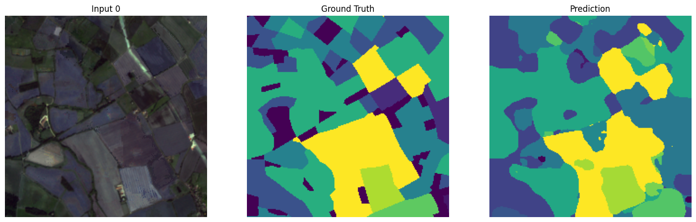

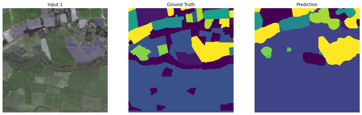
This visualisation presents the semantic segmentation predictions generated by the trained Prithvi-EO-2.0 model for a previously unseen batch of test images. As these images were not used during training or validation, they provide an unbiased assessment of the model’s ability to generalise to new data.

Each predicted segmentation map can be compared directly with the corresponding ground truth labels to assess how accurately the model identifies and delineates different crop classes. Areas where the predicted and ground truth maps closely align indicate successful classification, while discrepancies highlight regions where the model has confused visually similar crop types, struggled with underrepresented classes, or produced less precise field boundaries.

Conclusions¶

The results demonstrate that Prithvi-EO-2.0 can learn meaningful crop-specific representations from a relatively small labelled dataset. The final model achieved 66.2% overall accuracy, 53.9% mean Intersection over Union (mIoU), and a 66.9% macro F1 score across 16 crop classes. Performance was strongest for well-represented crop classes, while lower accuracy on several rare crop types highlighted the challenges posed by class imbalance. Overall, the results provide a promising proof of concept that geospatial foundation models can be effectively adapted for UK crop classification.