Example kittiwake: step 3.1 - seabORD run - distance decay
G_KI_run_decay.RmdBefore following this example, the model is assumed to be already calibrated. If not follow the article on calibration before running this example.
#use coastline
uk_map <- seabORD::cef_coast_4326


### theme definition
sysfonts::font_add_google("Montserrat", "montserrat")  # Base and heading font
sysfonts::font_add_google("JetBrains Mono", "jetbrains_mono")  # Code font
showtext::showtext_auto()

theme_bslib <- ggplot2::theme(
  plot.background = ggplot2::element_rect(fill = "#fff", color = NA),       # Background color
  panel.background = ggplot2::element_rect(fill = "#EAEFEC", color = NA),  # Panel background (secondary)
  panel.grid.major = ggplot2::element_line(color = "#EAEFEC"),             # Major grid lines
  panel.grid.minor = ggplot2::element_line(color = "#EAEFEC"),             # Minor grid lines
  axis.text = ggplot2::element_text(color = "#292C2F", family = "montserrat"),  # Axis text (foreground and font)
  axis.title = ggplot2::element_text(color = "#292C2F", family = "montserrat"), # Axis titles
  plot.title = ggplot2::element_text(color = "#0483A4", family = "montserrat", size = 16, face = "bold", hjust = 0.5), # Title
  legend.background = ggplot2::element_rect(fill = "#fff", color = NA),    # Legend background
  legend.key = ggplot2::element_rect(fill = "#EAEFEC", color = NA),        # Legend key
  legend.text = ggplot2::element_text(color = "#292C2F", family = "montserrat"), # Legend text
  plot.caption = ggplot2::element_text(color = "#292C2F", family = "jetbrains_mono"),
  axis.title.x = ggplot2::element_blank(),  # Remove x-axis label
  axis.title.y = ggplot2::element_blank(),# Caption for code font
)
Introduction & background
Now that we have run our calibration step and discerned the prey values resulting in moderate conditions in the absence of wind farms, we can continue with running the main SeabORD runs with matched pairs of baseline (no ORDs) and scenario (ORDs included).
This example
In this example we will run 1 scenario run (wind farm footprints included) with a prey value of 200.
Prepare inputs
For further information on inputs, please see Article “Example kittiwake: step 1 - seabORD inputs”.
This script will import the example parameters sets and spatial data, which are largely similar to the calibration inputs. Note will be given where these differ considerably, i.e., with regard to the inclusion of different wind farm footprints.
Parameter sets
Par_example <- seabORD::example_lists_dd$Par
str(Par_example) # view your list of main parameters - NOTE that $NScalefactor is now set to 1 meaning we are running with 100% of the populaution, which is customary for scenario runs.
#> List of 12
#>  $ thisSpecies        : chr "KI"
#>  $ colonies           : chr "UK9002491"
#>  $ Nscalefactor       : num 1
#>  $ Prob_Displacement  : num 0.6
#>  $ Prob_Barrier       : num 1
#>  $ PreyType           : chr "Uniform"
#>  $ collision          : chr "Off"
#>  $ SiteSelectionMethod: chr "Map"
#>  $ MaxDistancekm      : num 0
#>  $ PropInRange        : num 0
#>  $ Npairspercol       : num 2898
#>  $ Pmedian            : num 200

# Create the ouput folder "output_seabORD_scenario" specifically for scenario outputs if it doesn't alreay exist
if (!dir.exists("./output_seabORD_scenario")) {
  dir.create("./output_seabORD_scenario")
}

modPar_example <- seabORD::example_lists_dd$modPar
str(modPar_example) # We intend to run 5 replicates so need to change this in modPar
#> List of 5
#>  $ Nparallel  : logi NA
#>  $ initialseed: num 6598
#>  $ reference  : chr "serial_scenario_KI_UK9002491"
#>  $ outputdir  : chr "output_seabORD"
#>  $ Nreplicates: num 1
modPar_example$Nreplicates <- 1

# Lets check if this matches our prey values in Par_example
if (modPar_example$Nreplicates == length(Par_example$Pmedian)) {
  print("Nreplicates and number of prey inputs match - you may proceed")
} else {
  print("WARNING: Nreplicates and number of prey inputs DO NOT match - you may proceed, but will likely fail...")
}
#> [1] "Nreplicates and number of prey inputs match - you may proceed"

# # change our prey values in Par_example before we continue:
# Pmin <- 173  # min prey value from range determined in calibration
# Pmax <- 174  # max prey value from range determined in calibration
#
# # the following code will create a sequence spanning the range given:
# if (modPar_example$Nreplicates > 1){
#   Par_example$Pmedian <- seq(from = Pmin, to = Pmax, by = ((Pmax-Pmin)/(modPar_example$Nreplicates-1)))
# } else {
#   Par_example$Pmedian <- Pmax
# }
#
# # now check again:
# Par_example$Pmedian  # good to go!

modPar_example$outputdir  #this does not align with the directory created above
#> [1] "output_seabORD"
# so let's change it:
modPar_example$outputdir <- "output_seabORD_scenario"

ordPar_example <-  seabORD::example_lists_dd$ordPar
str(ordPar_example) # Including wind farms Nearth na Goithe and Inch Cape
#> List of 4
#>  $ include_ORDs   : chr [1:3] "Hywind Scotland Pilot Park" "Aberdeen Offshore W/F" "Kincardine"
#>  $ parnames       : chr "HYWD;ABDN;KINC"
#>  $ FootprintBorder: num 2
#>  $ BufferZone     : num 5

switches_example <- seabORD::example_lists_dd$switches
switches_example$savebirdflightmap <- TRUE # turn this switch on if you want to see an example of the birdflightmap output
switches_example$saverds <- TRUE
Assorted spatial inputs
Now load in all the spatial inputs. For more information please see the “Example kittiwake: step 1 - seabORD inputs” article.
example_data_seamask <- seabORD::seamask_3035_example

#make a raster with the right dimension/proj/extents etc.
seamask_example <-
  raster::raster(
    nrows = example_data_seamask$metadata[["n_rows"]],
    ncols = example_data_seamask$metadata[["n_cols"]],
    xmn = example_data_seamask$metadata[["x_min"]],
    xmx = example_data_seamask$metadata[["x_max"]],
    ymn = example_data_seamask$metadata[["y_min"]],
    ymx = example_data_seamask$metadata[["y_max"]],
    crs = example_data_seamask$metadata[["crs"]]
)

#fill it with the data available
seamask_example <- raster::setValues(seamask_example, #the raster
                                     example_data_seamask$matrix) #the values
#Set the name of the layer
names(seamask_example) <- "seamask_3035"


spadat1_example <-
  tibble::as_tibble( #as a tibble
      dplyr::filter(seabORD::spacoordinates, #the full dataset
                    SITECODE == "UK9002491") #the isle of interest
  )

spadat2_example <-
  tibble::as_tibble( #as a tibble
    dplyr::filter(seabORD::spalist, #the whole list
                  SITE_CODE == "UK9002491") #the site of interest
    )


# Overwite with the exact colony location of Whinnyfold used when creating map in step 1.1
spadat1_example$Longitude <- -1.85849
spadat1_example$Latitude <-  57.388807
spadat1_example$flt.LONG <- -1.85849
spadat1_example$flt.LAT <-  57.388807


spdat_example <-
   #tibble::as_tibble( #as a tibble
     dplyr::filter(seabORD::energeticsandpreydata,
                   Code == "KI")
    # )


example_data_brd_dd <- seabORD::BrdData_example_dd
#make the raster with the right dimensions..
BrdData_example_dd <-
  raster::raster(
  nrows = example_data_brd_dd$metadata[["n_rows"]],
  ncols = example_data_brd_dd$metadata[["n_cols"]],
  xmn = example_data_brd_dd$metadata[["x_min"]],
  xmx = example_data_brd_dd$metadata[["x_max"]],
  ymn = example_data_brd_dd$metadata[["y_min"]],
  ymx = example_data_brd_dd$metadata[["y_max"]],
  crs = example_data_brd_dd$metadata[["crs"]]
)
#fill it with the data
BrdData_example_dd <- raster::setValues(BrdData_example_dd,
                                     example_data_brd_dd$matrix)
#Set the name of the layer
names(BrdData_example_dd) <- "Whinnyfold"


example_data_frg_dd <- seabORD::frgcompdata_example_dd
#make the raster with the right dimensions..
FrgCompData_example_dd <-
  raster::raster(
  nrows = example_data_frg_dd$metadata[["n_rows"]],
  ncols = example_data_frg_dd$metadata[["n_cols"]],
  xmn = example_data_frg_dd$metadata[["x_min"]],
  xmx = example_data_frg_dd$metadata[["x_max"]],
  ymn = example_data_frg_dd$metadata[["y_min"]],
  ymx = example_data_frg_dd$metadata[["y_max"]],
  crs = example_data_frg_dd$metadata[["crs"]]
)
#fill it with the data
FrgCompData_example_dd <- raster::setValues(FrgCompData_example_dd,
                                         example_data_frg_dd$matrix)
#Set the name of the layer
names(FrgCompData_example_dd) <- "Whinnyfold"


UK9002491_bysea <- seabORD::UK9002491_bysea_3035
#make the raster with the right dimensions..
fltdist_base_example <-
  raster::raster(
  nrows = UK9002491_bysea$metadata[["n_rows"]],
  ncols = UK9002491_bysea$metadata[["n_cols"]],
  xmn = UK9002491_bysea$metadata[["x_min"]],
  xmx = UK9002491_bysea$metadata[["x_max"]],
  ymn = UK9002491_bysea$metadata[["y_min"]],
  ymx = UK9002491_bysea$metadata[["y_max"]],
  crs = UK9002491_bysea$metadata[["crs"]]
)
#fill it with the data
fltdist_base_example <- raster::setValues(fltdist_base_example,
                                          UK9002491_bysea$matrix)
#as a raster brick. #WHY? only one layer
fltdist_base_example <- raster::brick(fltdist_base_example)
#Set the name of the layer
names(fltdist_base_example) <- "UK9002491"


FlightGridcorrection <- seabORD::FlightGridcorrection_3035

ORDpoly_example <- seabORD::ORDpoly_example_wfold # commented out as not required for calibration runs
You can plot the ORD footprints for peace of mind:
ORDpoly_example_repr <- ORDpoly_example %>%
  sf::st_transform(sf::st_crs(uk_map))

ggplot2::ggplot() +
  # Plot the reprojected UK map in red
  ggplot2::geom_sf(data =  uk_map, fill = NA, color = "#D63333", size = 1.5) +
  # Add the ORDpoly_example shapes with a different color
  ggplot2::geom_sf(data = ORDpoly_example_repr, fill = "#0483A4", color = "#0483A4", size = 1) +
   ggplot2::coord_sf(
    xlim = c(-3, 0.5),  # Longitude range (adjust as needed)
    ylim = c(56.25, 58.25)     # Latitude range (adjust as needed)
  ) +
  theme_bslib +  #palette theme
  ggplot2::labs(title = "coasts (red) and ORDpoly (blue)")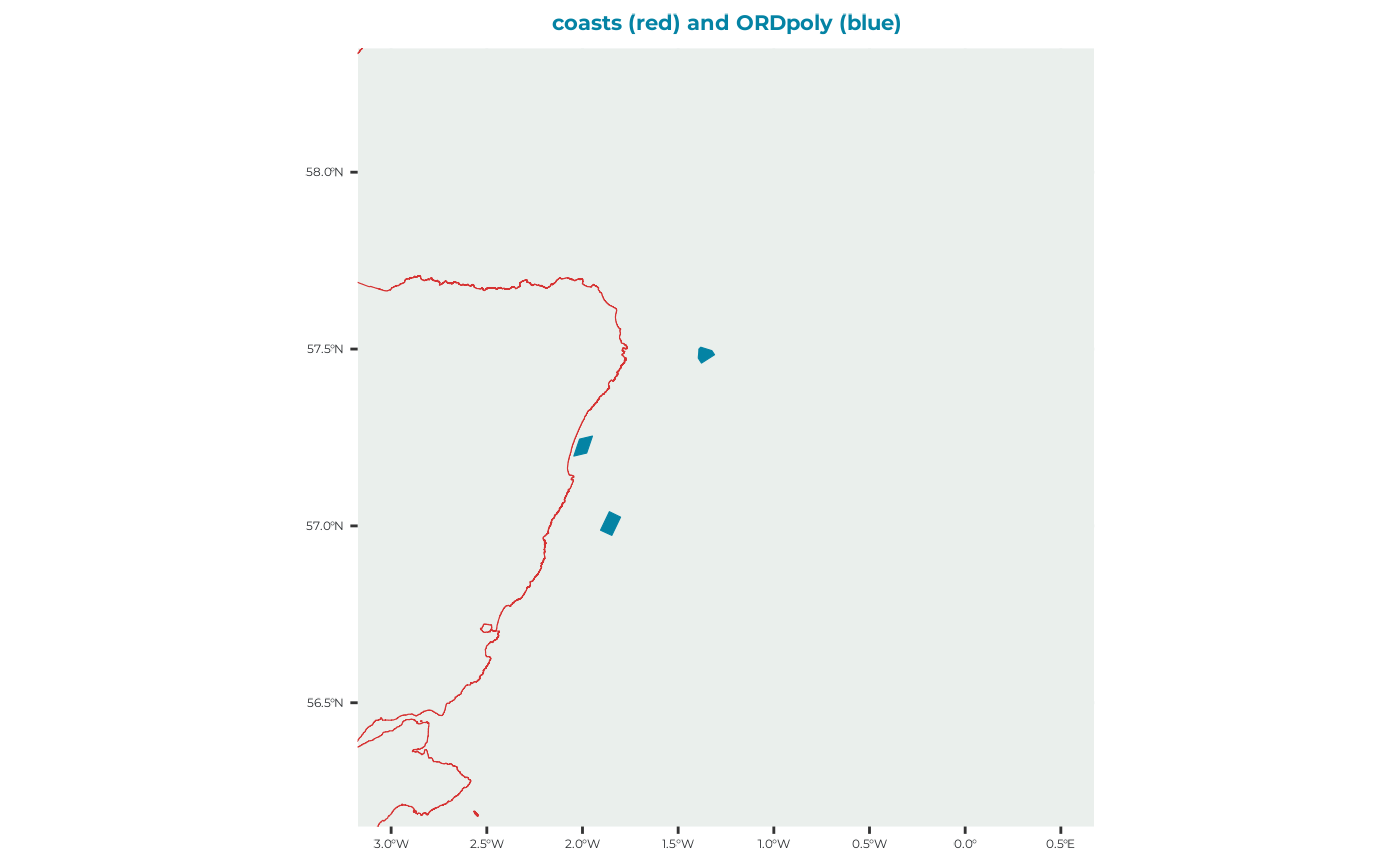
Running seabORD
Now that all the inputs are ready we can run the model using:
# SeabORDoutput <- seabord(Par = Par_example,
#                          ordPar = ordPar_example,
#                          modPar = modPar_example,
#                          switches = switches_example,
#                          seamask = seamask_example,
#                          spadat1 = spadat1_example,
#                          spadat2 = spadat2_example,
#                          spdat = spdat_example,
#                          BrdData = BrdData_example,
#                          FrgCompData = FrgCompData_example,
#                          fltdist_base = fltdist_base_example,
#                          FlightGridcorrection = FlightGridcorrection,
#                          ORDpoly = ORDpoly_example)
#
# # Save SeabORDsummary:
#  if (switches_example$saverds) {
#     saveRDS("SeabORDoutput", file.path(modPar_example$outputdir, paste0("sb_out_", gsub("\\.", "_", make.names(paste0(modPar_example$reference,"_", Sys.Date()))),".rds")))
# }
SeabORD runs including wind farms and full populations can take a while to run - even with a relatively small population of ~ 3,000 pairs.
The output will be saved in in your output directory set up in modPar.
To learn more about the main functions behind seabORD you can read the article on the main functions
To see how you can read in and plot the results you can read the article “Example kittiwake: step 4 - interpreting the outputs” where we have an example output for you to play with.