Section 17 Comparison of Data Sources
17.1 Results
Having assembled all the available data sources, we can now plot them on a common series of axes to compare their absolute magnitudes and relative trends in time.
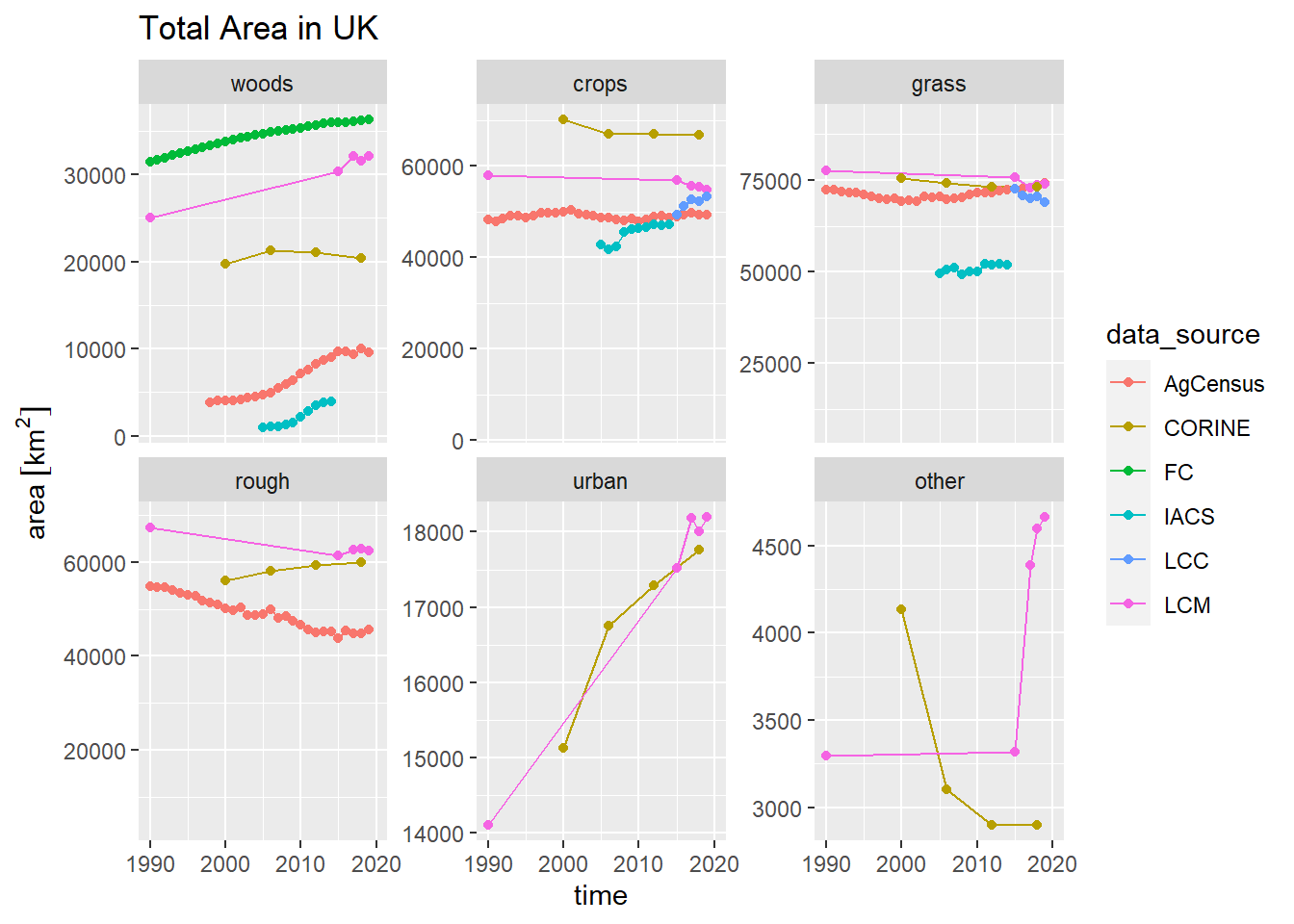
Figure 17.1: Time series of land-use areas \(\mathbf{A}\) observed by different data sources. Note that IACS data only cover England, so are included for comparison of trends only.
Figure 17.1 shows the total areas of each land-use class estimated by the available data sources. For the total area of woodland, Agricultural Census and IACS only record the woodland area occurring on agricultural land, so these should not be expected to match the actual totals; they are only included to compare the rate of increase. However, between the remaining sources, there is a wide range in estimates, varying by 16000 km2, with FC > LCM > CORINE. CORINE shows an apparent decline in woodland area, which has to be considered suspect. LCM and FC show similar trends, but LCM estimates the woodland area to be ~ 6000 km2 lower. Because the FC data is largely based on ground-based survey and aerial photography rather than satellite, we assume this to be more reliable.
The Agricultural Census shows the total crop area to be relatively stable at ~50000 km2. The latter part of the IACS data appear in close agreement with this, but they account only for England. Adding in the crop area of Scotland, Wales and NI suggests that the IACS estimates exceed the Agricultural Census by around 10000 km2. The IACS crop data show a step change after the first three year, which is probably an artefact of changes in the methodology of IACS reporting. The LCC data start in close agreement with Agricultural Census, but show a strongly rising trend of ~5000 km2 not seen in other data sources. Both CORINE and LCM show higher crop areas, with a declining trend not seen in the ground-based data.
For grassland, the outlying line of IACS data can be discounted as it covers only England, and is included only for comparison of trends. Otherwise, estimates seem in closer agreement in absolute terms, although trends are not very consistent across data sources. The total area of rough grazing and semi-natural land shows a similar decline in both Agricultural Census and LCM, although their initial starting points differ by 10000 km2. CORINE shows the reverse, which appears implausible. For urban and built-up land however, LCM and CORINE show very close agreement on the absolute area and trend. Estimates of the total area of other land uses are only provided by LCM and CORINE, and neither appears plausible as genuine land-use change. This other land is mostly coastal zone, and it is more likely that this apparent change is due to differences in satellite imagery and the algorithms used to classify them.
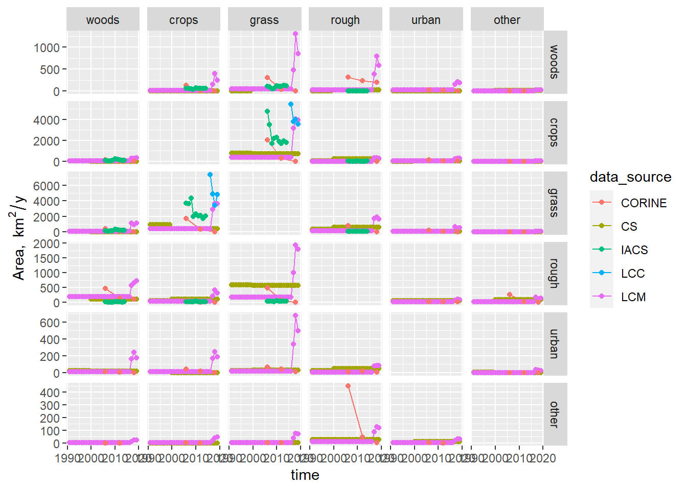
Figure 17.2: Time series of area changing from each land use to every other land use (the matrix \(\mathbf{B}\)) observed by different data sources. LCM and CS values between surveys were interpolated values as constant annual rates.
Figure 17.2 shows the \(\mathbf{B}\) matrix over time. The y axis scales are somewhat skewed by a number of outlying high values. The plots on the top row, representing deforestation, are dominated by the high values from post-2015 LCM. Given the abrupt change with the previous LCM estimate, these would seem implausible. For the conversions from crop to grass and vice versa, the LCC and post-2015 LCM data give very high values (4000 to 6000 km2) compared with CS and pre-2015 LCM (< 500 km2). IACS also shows similarily high values when we account for the fact that this only cover England and also with a step-change in the time series that appears implausible. Similar patterns are seen in other panels e.g. other to rough, where a single CORINE value dominates. Because of these order-of-magnitude differences, it is hard to discern subtler features here. As an alternative presentation, we can show the matrix numerically, with the colour scale indicating the magnitude of the area (Figure 17.3).
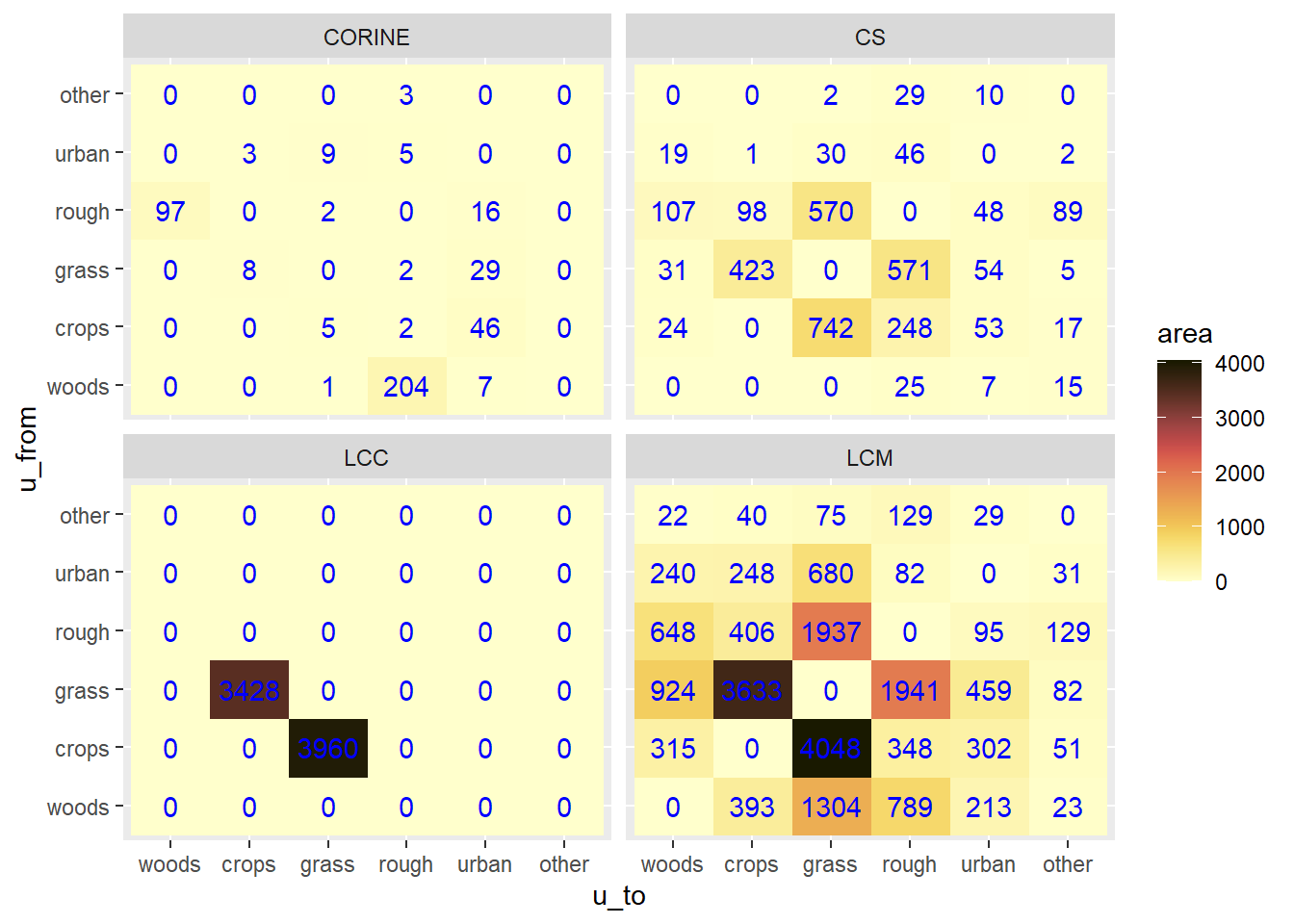
Figure 17.3: Area changing from each land use to every other land use (the matrix \(\mathbf{B}\)) observed by different data sources between 2017 and 2018.
Figure 17.3 indicates that LCC and LCM give \(B\) values that are approximately an order of magnitude higher than CS and CORINE in 2017-2018. The former give crop-grass transitions close to 4000 km2; CS averages 583 km2. For grass-rough transitions, LCM gives values close to 2000 km2; CS estimates 570 km2. To examine the general patterns over time more clearly, we can plot the gross changes of each land-use class i.e. the sums of the rows and columns in Figures 17.4 and 17.5.
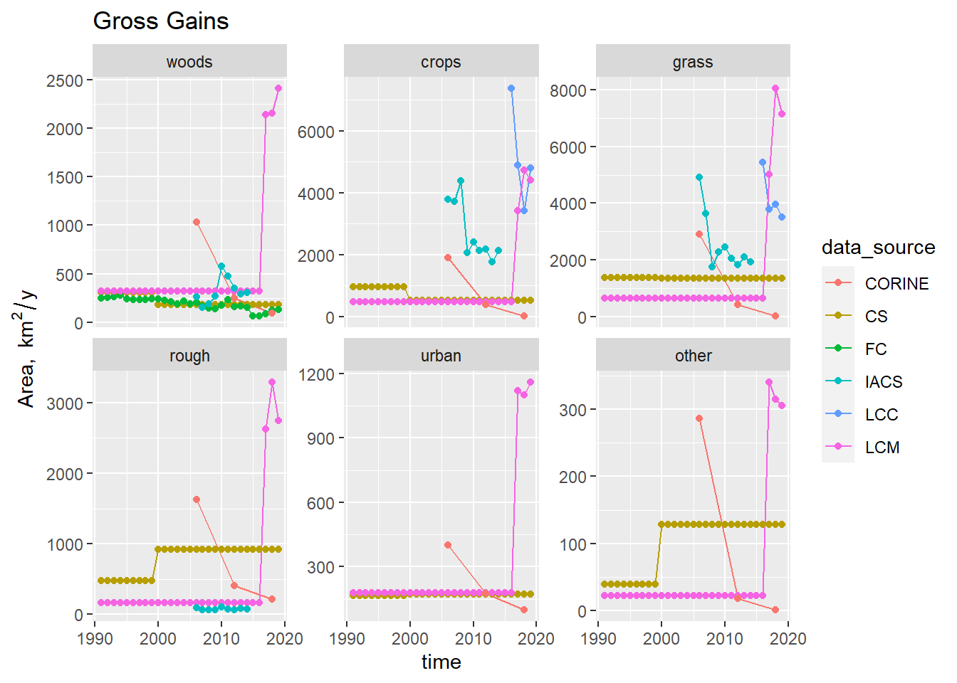
Figure 17.4: Time series of gross gain of area \(\mathbf{G}\) to each land use observed by different data sources. LCM and CS values between surveys were interpolated values as constant annual rates.
Figure 17.4 shows the gross gain in area of each land use. For woodlands, we would place highest confidence in the FC data (green symbols), which shows the gross gain to have declined from 250 km2 to near zero in 2016. The 1990-2015 LCM data gives a slightly higher mean compared to this, and the CS data are not truly independent of the FC data as they share some data in common. The post-2015 LCM data show much higher rates, over 2000 km2, which are not believable. CORINE also shows high afforestation in 2006, but sharply declining; again this is not believable, assuming the FC data are resonably reliable.
A similar lack of agreement is generally apparent in the data for the other five land uses. The 1990-2015 LCM and CS data show reasonable agreement The post-2015 LCM, LCC and IACS data show much higher gross gains. In the case of crops, if we factor in that the IACS data only account for England, then these three data sets are in some agreement that the gross gain in crop is in the range 3000-7000 km2. However, their patterns over time make us suspicious of their validity. The large year-to-year variability seems unlikely, and the patterns in LCC and LCM are not consistent.
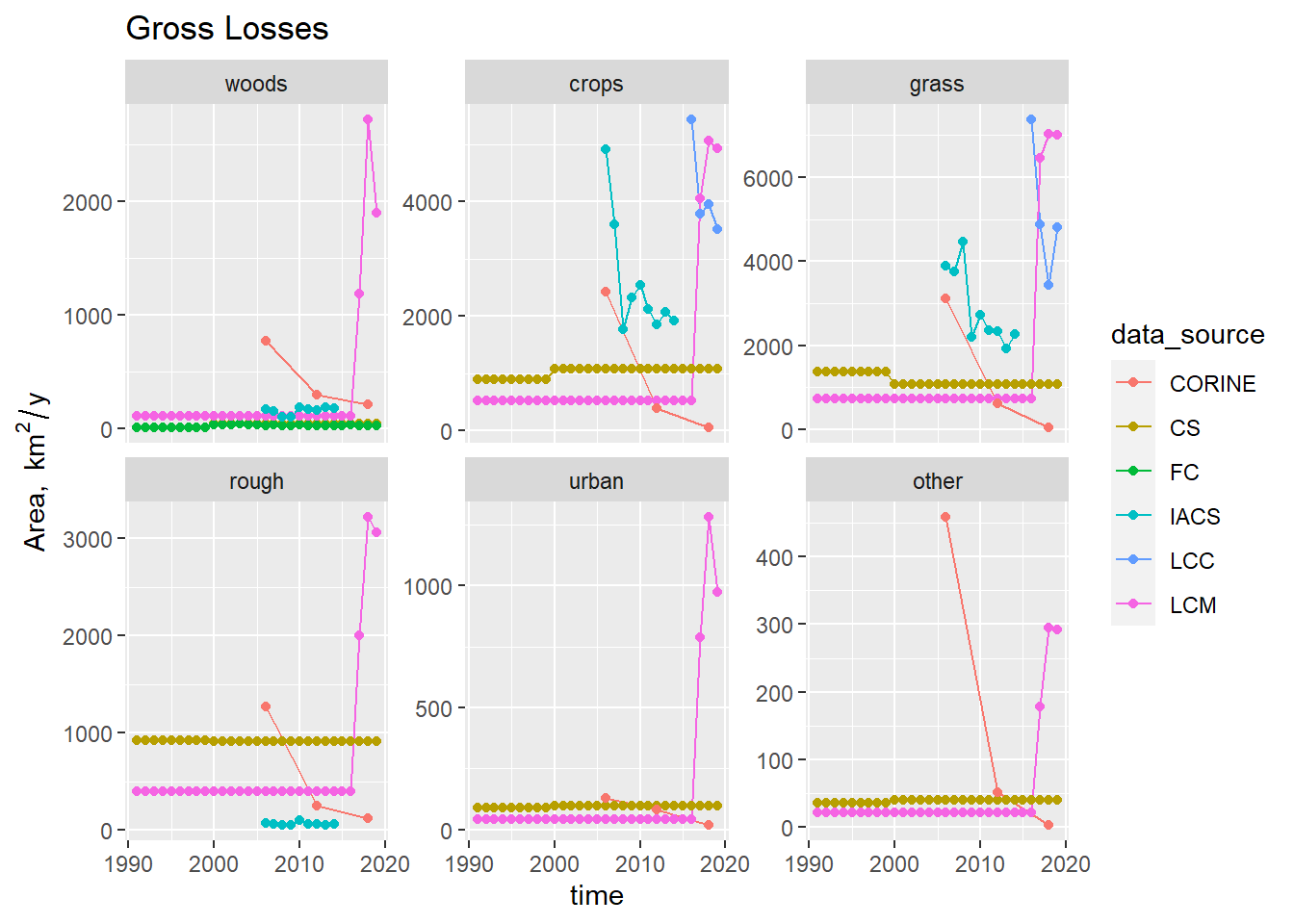
Figure 17.5: Time series of gross loss of area \(\mathbf{L}\) from each land use observed by different data sources. LCM and CS values between surveys were interpolated values as constant annual rates.
Examining the gross losses shows a similar picture(Figure 17.5). According to FC data (green symbols), deforestation rates have remained very low, less than 50 km2. The 1990-2015 LCM data gives a close but slightly higher mean compared to this. The post-2015 LCM data show much higher rates, over 2000 km2, which again seem implausible. CORINE also shows high deforestation in 2006, which then decreses. Over all land uses, there is essentially the same overall pattern as in the gross gains. with the 1990-2015 LCM and CS data showing small losses, whilst the post-2015 LCM, LCC and IACS data show much larger losses.
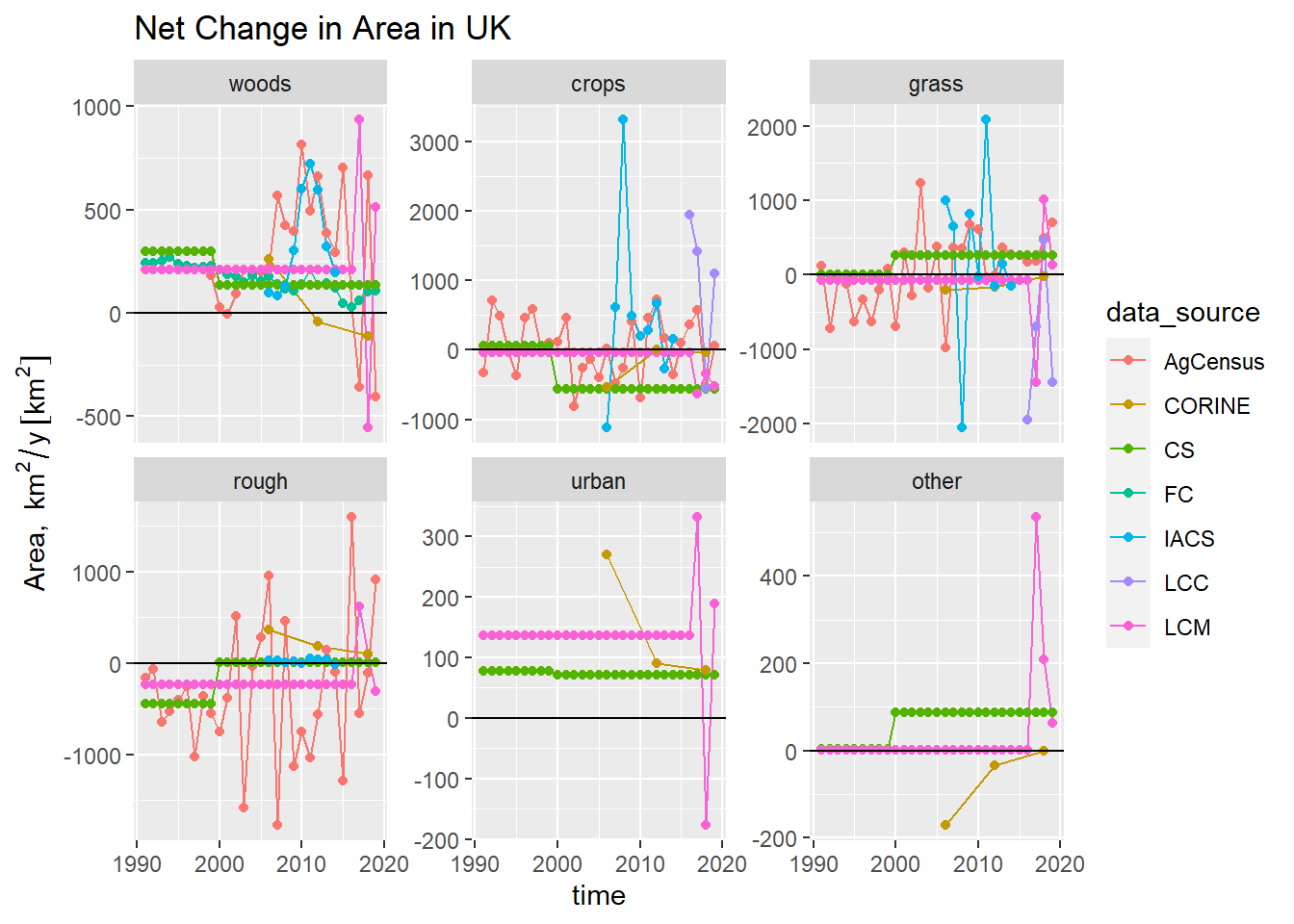
Figure 17.6: Time series of net change in area of each land use \(\Delta \mathbf{A}\) observed by different data sources.
The net effect of these gains and losses is shown in Figure 17.6. The same broad pattern is apparent The 1990-2015 LCM and CS data give lower estimates, with little temporal resolution because of the frequency of the surveys. The Agricultural Census shows annual variability, oscillating from positive to negative, but at a lower level. LCC, post-2015 LCM data, and IACS data show higher net rates of change, with rates of net change 3-4 times higher and a more noisy pattern.
17.2 Discussion
From the above results, it appears that more work remains to be done on the EO-based data sets before they are suitable for use as direct measures of land-use change. Whilst the larger gross changes that they observe may be correct, their patterns over time make them appear less plausible. Particularly, the temporal patterns are not consistent (i.e. they do not increase and decrease at the same times), and the large year-to-year variability seems unlikely, given the way land management works. It appears that their sensitivity for detecting change alters over time. In the CORINE time series, both the gains and losses are initially large, and both decline at a similar rate over time. not useful. With LCM, there is a clear difference between the magnitude of gross change detected in recent years compared with pre-2015. The IACS data are also not consistent in time, and the magnitude and variability of changes appears questionable.
None of the data sources here represent absolute truth. We cannot rule out the possibility that the much higher gross change rates are indeed correct, and that the Agricultural Census and CS underestimate these. However, we should consider other factors as well as the patterns in the data themselves. Firstly is the parsimony principle: if small gross changes can reproduce the observed net change, this is fundamentally more more probable than the occurence of large gross changes, all else being equal. In the Bayesian methodology, we can specify this as a prior probability distribution, and the the extent to whether “all else” really is “equal” is quantified by the observed data. We use this approach later. Secondly, the errors produced by EO-based and ground-based estimates are quite different. If we estimate land-use change by differencing maps, errors in the maps appear as spurious land-use change. So this method will necessarily over-estimate land-use change, to an extent that can be predicted from the predictive accuracy of the individual maps. The error variance in the land-use change estimate will be the sum of the variance in the two maps used. Future work may provide a quantification of this. The systematic errors present in ground-based estimates are less clear-cut, as it depends on the methodology used. However, because it requires sampling effort to detect change, it is commonly assumed that it is easier to under-estimate change. Again, future work may clarify this.
Given the uncertainties in the EO data that may be tackled at a later stage, we focus on using ground-based observations for the data assimilation in WP-A, as originally proposed. We elect to use CS, FC and Agricultural Census data to estimate the \(B\) matrix. We use the spatial pattern in the other data sources (LCM, LCC, IACS, CORINE) to estimate the likelihood of where change occurs, but not in the estimation of the \(B\) matrix itself. This is a conservative approach, as the emphasis is on the same input data sets as used in the current inventory method, but constrains them with the net change measured by the national-scale Agricultural Census data, and the spatial pattern contained in LCM, LCC, IACS, and CORINE data. In this way we can try to minimise confounding changes to the methodology for estimating land-use change, and the data sources used in its estimation.
The issues with the time trends and the plausibility of much higher gross rates of change in these data sets are issues which may be resolved in future work, which will focus on EO data. There are various approaches to further examining this. For example, if the IACS data are reliable, they should match the spatial pattern in the Agricultural Holdings data. If the two data sets are at odds, we cannot have great confidence in both of them. The Agricultural Census contains some data which would act as a constraint on our estimates of the gross changes to/from grass. The area of grassland less than five years old is specified. Assuming a uniform distribution, one fifth of this would be converted each year on average, which would give a ball-park estimate of the gross gain and loss. The complications arise in the age distribution of grassland (what area is > 5 years old?) and whether the distribution is really uniform. Lastly, some other data sets exist for comparison, but have not become available within the time frame of this project (further IACS data, CROME, and LUCAS).