Section 19 Estimating \(B\) by MCMC
19.1 Introduction
As described in the Methods section, we perform the data assimilation (DA) as a two-stage procedure. The previous section showed how the first stage can be done in a simple way with least-squares optimisation. In this section, we re-do the data assimilation using a Bayesian approach. The aim is to find not only the \(B\) matrix parameters with the maximum likelihood, but also the full posterior distribution for the parameters and predictions. This quantifies the uncertainty in our estimates and predictions of land-use change. To do this, we use a Markov chain Monte Carlo (MCMC) algorithm. MCMC is the standard method for Bayesian parameter estimation where the problem is too complex for an analytical solution to be found. It provides a means of sampling from an unknown posterior distribution, so long as the likelihood of the data can be evaluated.
19.2 Methods
The method used here closely follows that described by Levy et al. (2018), so our description here is brief, and focuses on the relatively minor differences.
19.2.1 Observational data
Based on the earlier discussion of data sources, we elected to use CS, FC and Agricultural Census data to estimate the \(B\) matrix. Other data sources can be still used to estimate the spatial pattern in land-use change, and can be added to the estimation of the \(B\) matrix in future. At present, the other data sources examined were either inconsistent in quality and the focus of ongoing and future work, incomplete, or unequivocal permission for use had not been obtained.
19.2.2 The model
The model used here is the simple arithmetic of matrices described in the Methods section. Given a matrix \(B\), this calculates the gross and net changes in area \(G, L\) and \(\Delta A\). The only additional element, which is simple but potentially confusing for terminology, is that as well as the \(B\) values acting as parameters, we also have observations of these, and this comparison is included in the likelihood. In mathematical terms, we can think of this part of the model as being the identity function, i.e. a function which returns the input value, so \(y = f(B) = B\).
19.2.3 Prior distributions
Levy et al. (2018) used the CS data as the prior distribution for the \(B\) matrix. This made sense in that context, where there were more data sources available, and CS had been used as the basis for previous estimates. In the present case, in order to treat all the data sources consistently, it is easier to consider this as an observational data set like the others. We then need to specify a prior distribution for \(B\) independently of the data. We chose two options for comparison (Figure 19.1):
- a uniform distribution, where all \(B\) parameters could vary between 0 and 10000 km2, and
- a half-normal distribution, with mean zero and standard deviation \(\sigma = 3000\) km2. “Half-normal” means that only positive values are possible. This provides a relatively weak version of the parsimony principle, that lower rates of gross change are more probable (all else being equal). The strength of this assumption can be altered by varying \(\sigma\).
Large differences were not seen between these two, and all results shown here use only the uniform prior assumption for simplicity, though there is scope for further exploration here.
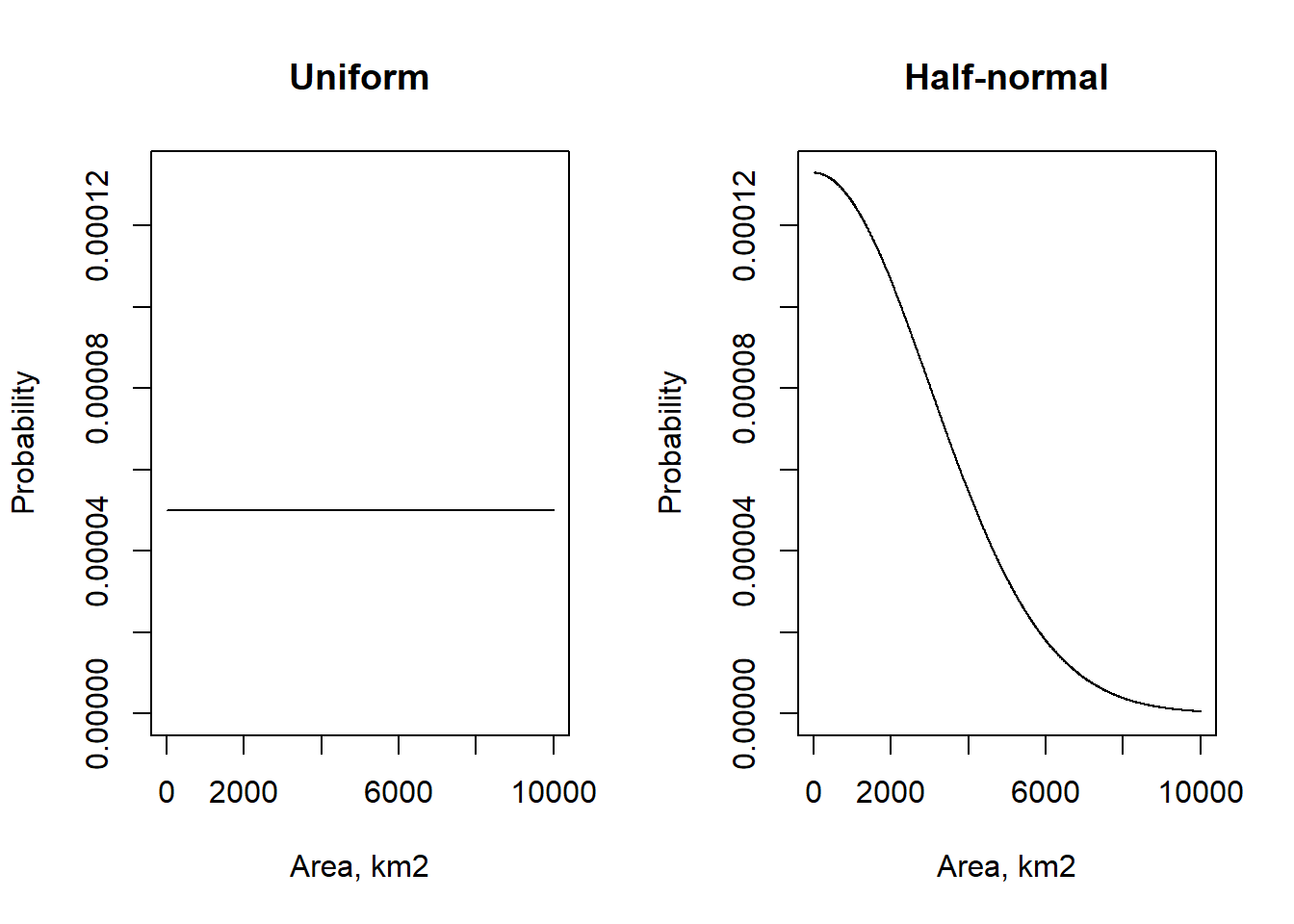
Figure 19.1: Two alternative prior distributions for the \(B\) parameters.
19.2.4 Likelihood function
The likelihood function is very similar to the function used to calculate RMSE in the previous section.
The key difference is that, for each observation, a likelihood is calculated, assuming that measurement errors show a Gaussian distribution (hence the use of the dnorm function) and are independent of each other.
To put this in mathematical notation, the likelihood of observing the net change \(\Delta A^{\mathrm{obs}}\) is
\[\begin{equation} \label{eq:likNet} \mathcal{L} = \prod_{\substack{u=1}}^{\substack{n_u}} \frac{1}{\sigma_{u}^\mathrm{obs} \sqrt{2\pi}} \mathrm{exp}(-(\Delta A_{u}^{\mathrm{obs}} - \Delta A_{u}^{\mathrm{pred}})^2/2 {\sigma_{u}^\mathrm{obs}}^2) \end{equation}\]
where \(\Delta A_{u}^{\mathrm{pred}}\) is the prediction for the change in land use \(u\), given the parameter matrix \(\mathbf{B}\), and \(\sigma_{u}^\mathrm{obs}\) is the measurement uncertainty. There are analagous terms for \(G, L\) and \(B\) which can all be multiplied.
Rather than assume that measurement uncertainty is the same for all observations, we specify that it is proportional to the \(y\) value. That is, observations of large areas come with larger absolute uncertainty. Potentially, we can specify unique uncertainties for each data source and observation. At present, we do not have a basis for specifing these uncertainties based on a proper quantitative analysis, but this could be an area of future work. For now, we assume that all data sources are equal, and assign them the same relative uncertainty.
19.2.5 MCMC algorithm
Many MCMC algorithms are available.
We chose the parallelised version of the DiffeRential Evolution Adaptive Metropolis or “DREAMz” algorithm (Vrugt et al. 2008), a development of an earlier Differential Evolution algorithm (ter Braak and Vrugt 2008). These, and other MCMC algorithms are implemented in the R package BayesianTools (Hartig, Minunno, and Paul 2017), which allowed us to compare the efficiency of different approaches.
Differential Evolution MCMC uses an adaptive algorithm, in which multiple chains are run in parallel.
It uses information from the past states of multiple chains, by generating jumps from differences of pairs of past states.
It increases efficiency, particularly for high-dimensional problems, producing convergence with fewer iterations and fewer chains, estimated to be about 5–26 times more efficient than the typical Metropolis sampler (ter Braak and Vrugt 2008).
The problem was parallelised at two levels. Firstly, we can parallelise in the time dimension. The transition matrix between each pair of years can be treated independently, so we can run all years on separate processors at the same time. In other words, we treat the time series between 1990 and 2019 as 30 separate tasks, rather than one. Secondly, we can parallelise across MCMC chains. The DREAMz algorithm uses multiple chains, each with a number of internal chains which inter-communicate. So long as we allow for this inter-communication, we can run each (internal) chain on a separate processor. For each pair of years, we ran 120000 iterations with nine chains in total (three chains, each with three internal chains). Running a single chain of this type takes around 10 mins. If we ran all nine chains for 30 years in series, this would take 30 x 9 x 10/60 = 45 hours. Using 270 processors on the NERC/STFC JASMIN super-computer, all chains can be run simultaneously in ten minutes, subject to the job queueing system having capacity.
19.3 Results
Figure 19.2 shows the basic diagnostic check for MCMC output. The chains should start over-dispersed, so that a wide range of parameter space is explored. After a “burn-in” phase, the chains should begin to converge on an area of high probability. To account for auto-correlation between sequential samples, it is standard practice to “thin” the chains by a factor of ten or more, i.e. leaving only every tenth value. Here, the iteration count refers to the thinned samples, so the actual iteration count is a factor of ten higher. Depending on the nature of the model and the data, we might expect something like a normal distribution around the most likely value, though this is not necessarily the case. The diagnostic test for convergence is whether the variation among chains is greater than the variation within chains, and we reach this point after about 4000 thinned iterations.
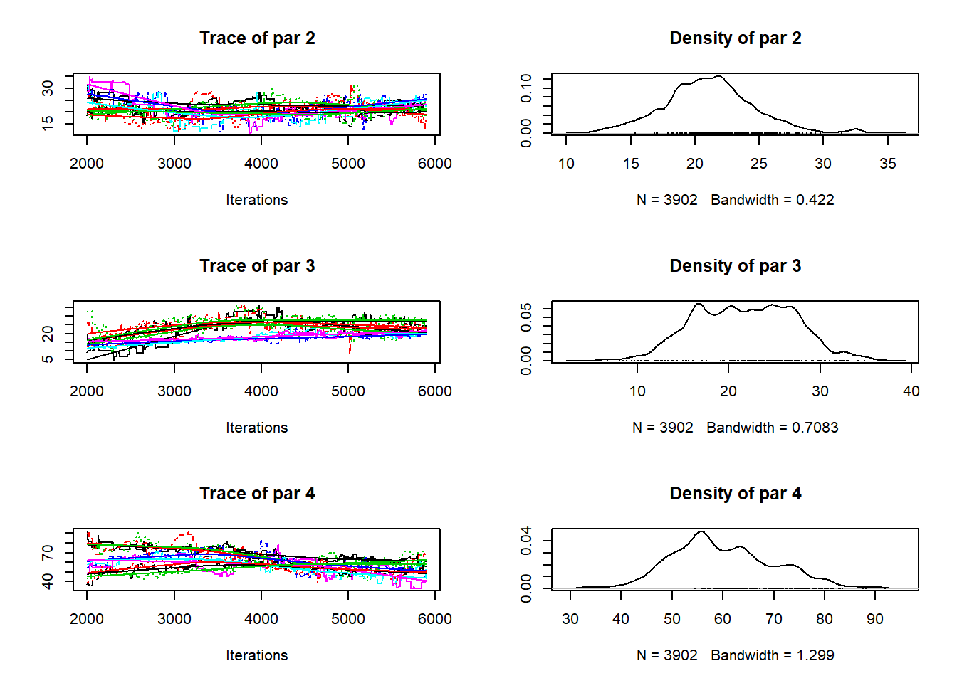
Figure 19.2: Trace plots for three parameters from the MCMC run for 2018-2019. Parameters represent the area changing from woods to crop, grass and rough grazing, respectively. The left-hand plot shows the values sampled from the posterior as the iterations progress in each chain. Different colours show the different MCMC chains. The iteration count refers to the thinned samples after burn-in; the actual iteration count is a factor of ten higher. The right-hand plot shows the density distribution of parameter values, which represents our sampled approximation to the posterior probability distribution.
An important feature of the MCMC approach is that it properly estimates the joint probability distribution for the parameters, and these correlations are automatically incorporated. In the example shown in Figure 19.3, the areas changing from crop to grass and vice versa are clearly positively correlated. This follows because the net change is constrained by the observations; if the crop-to-grass area is large, the grass-to-crop area also has to be large to fit with the observed net change.
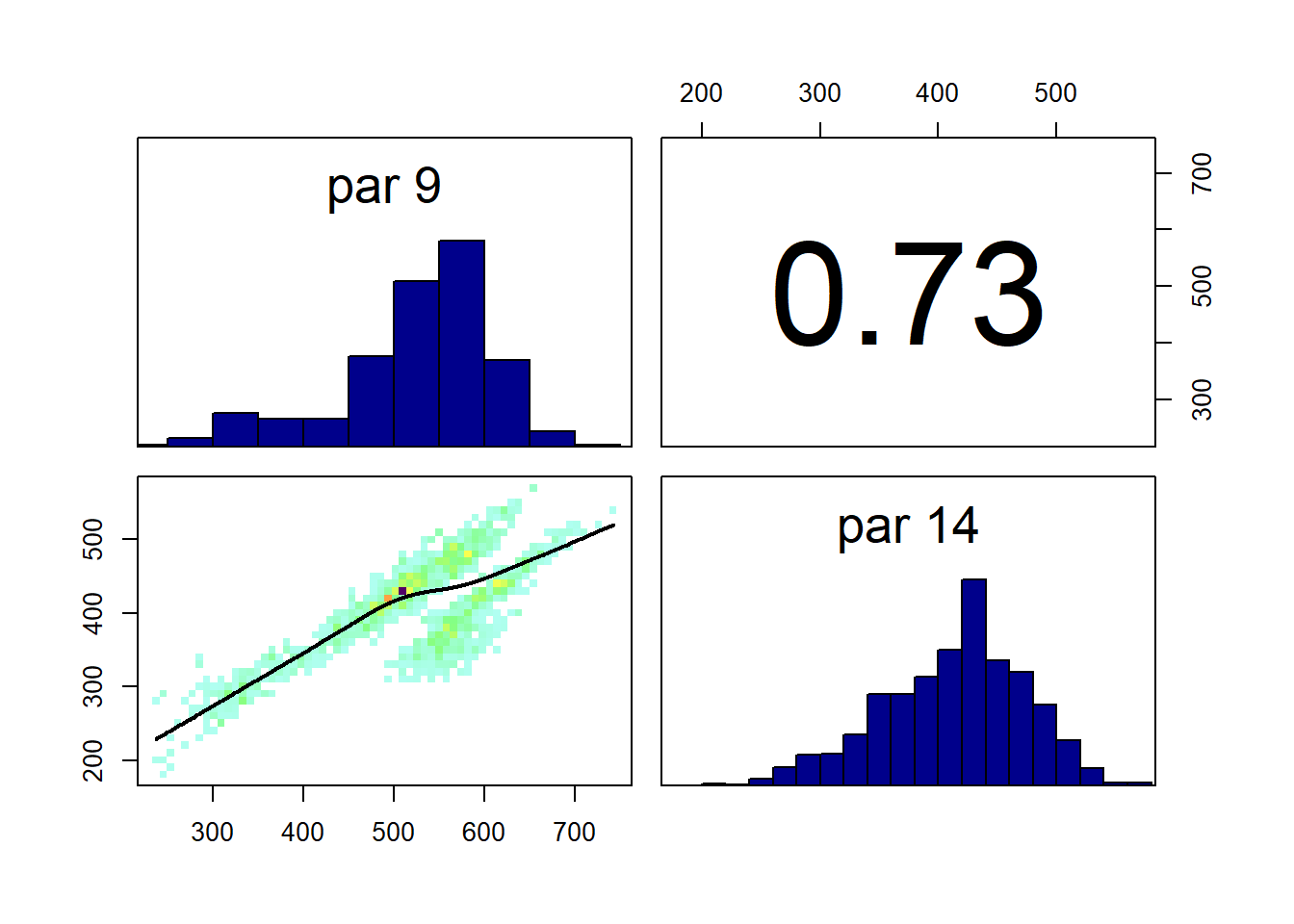
Figure 19.3: Correlation plot for two parameters from the MCMC run for 2018-2019. Parameters represent the area changing from crop to grass and vice versa. The plot shows the correlation between parameters values obtained over the course of the MCMC sampling. This represents our sampled approximation to the correlations in the joint posterior probability distribution for the parameters.
In Figures 19.4, 19.5, 19.6, and 19.7, the solid red line shows the maximum a posteriori estimate, which represents the \(B\) parameter set with the highest posterior probability, the closest equivalent to a “best-fit” estimate. The shaded area denotes the 95 % credibility interval. In these plots, the MCMC estimates do not fit any single set of observations or the \(B, G, L\) or \(\Delta A\) variables exactly, as they are constrained by all of these simultaneously.
Figure 19.4 shows the time course of the posterior distribution of the \(B\) matrix estimated by MCMC. The estimates are strongly influenced by the CS data, as these provide the only observations of \(B\) used here. However, annual variability is introduced, as the parameters are varied to simultaneously fit with the Agricultural Census and FC data. In most cases, the posterior estimates fit closely with the CS observations but this is not always the case. To understand the deviations and cause of year-to-year variability is not easy, because this is a very high-dimensional problem. For example, the \(B\) parameter for the transition woods-to-rough is lower and more variable than the CS observation after 2000. However, the likelihood of this parameter is influenced by the agreement with all the other observations and variables. The MCMC algorithm attempts to find parameter sets which simultaneously satisfy all the conditions described by the observations e.g. that the area changing from woods-to-rough is a constant 25 km2 (CS); that the total gains and losses to/from rough are close to 1000 km2 (CS); and that the net change in rough grazing varies between +1500 km2 and -1500 km2 over the same period (Agricultural Census).
In the case of forestry, where we have the observations of the gross gains and losses, the problem is much better constrained (Figures 19.5 Figure and 19.6) . Here, the posterior estimates fit the FC and CS estimates well, but cannot simultaneously reproduce the pattern in the Agricultural Census data (Figure 19.7, top left). The Agricultural Census data, clearly have an influence on the year-to-year pattern in the estimates, but parameter combinations which would reproduce the amplitude of variation seen in the Agricultural Census data clearly have lower likelihood.
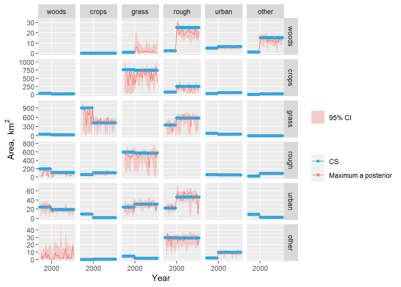
Figure 19.4: Observations and posterior distribution of the transition matrix \(\mathbf{B}\), representing the gross area changing from the land use in each row to the land use in each column each year from 1990 to 2019. The shaded band shows the 2.5 and 97.5 percentiles of the posterior distribution. The maximum a posteriori estimate is shown as the solid red line within this. Note the y scale is different for each row.
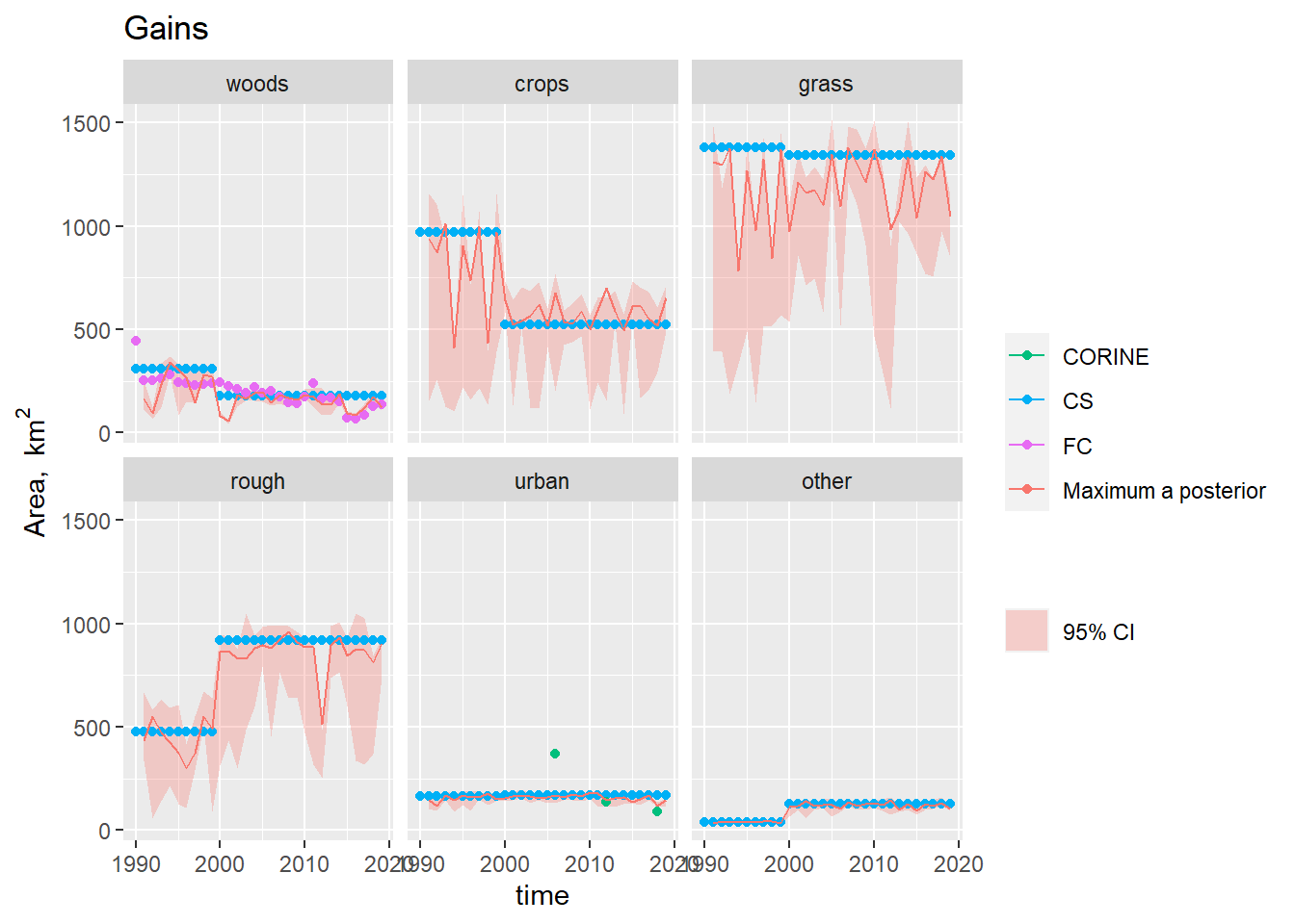
Figure 19.5: Observations and posterior distribution estimated by MCMC of the gross gain in area of each land use \(\mathbf{G}\) from 1990 to 2019. The shaded band shows the 2.5 and 97.5 % percentiles of the posterior distribution. The maximum a posteriori estimate is shown as the solid red line within this.
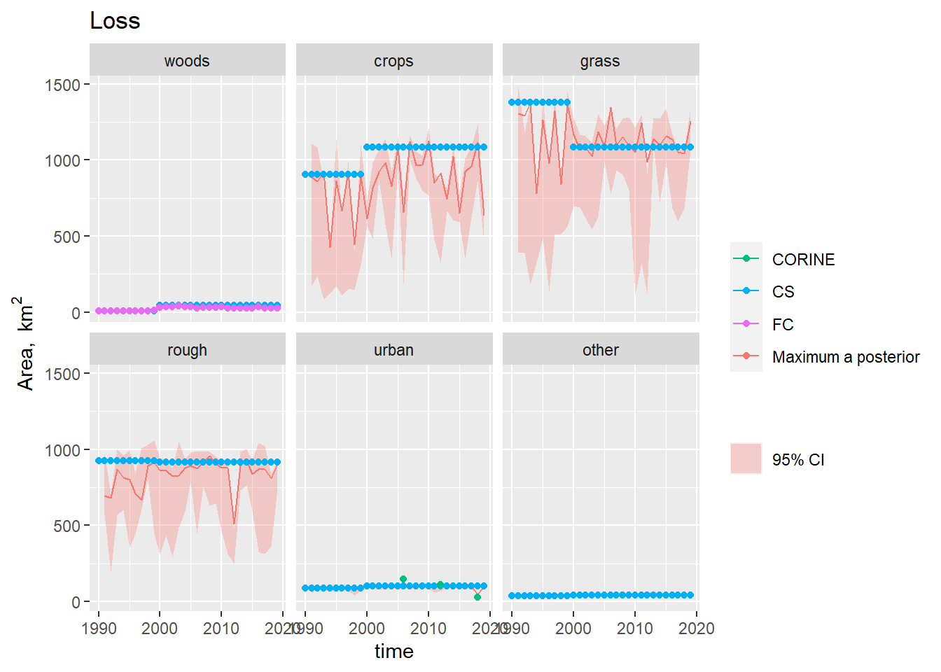
Figure 19.6: Observations and posterior distribution estimated by MCMC of the gross loss of area from each land use \(\mathbf{L}\) from 1990 to 2019. The shaded band shows the 2.5 and 97.5 % percentiles of the posterior distribution. The maximum a posteriori estimate is shown as the solid red line within this.
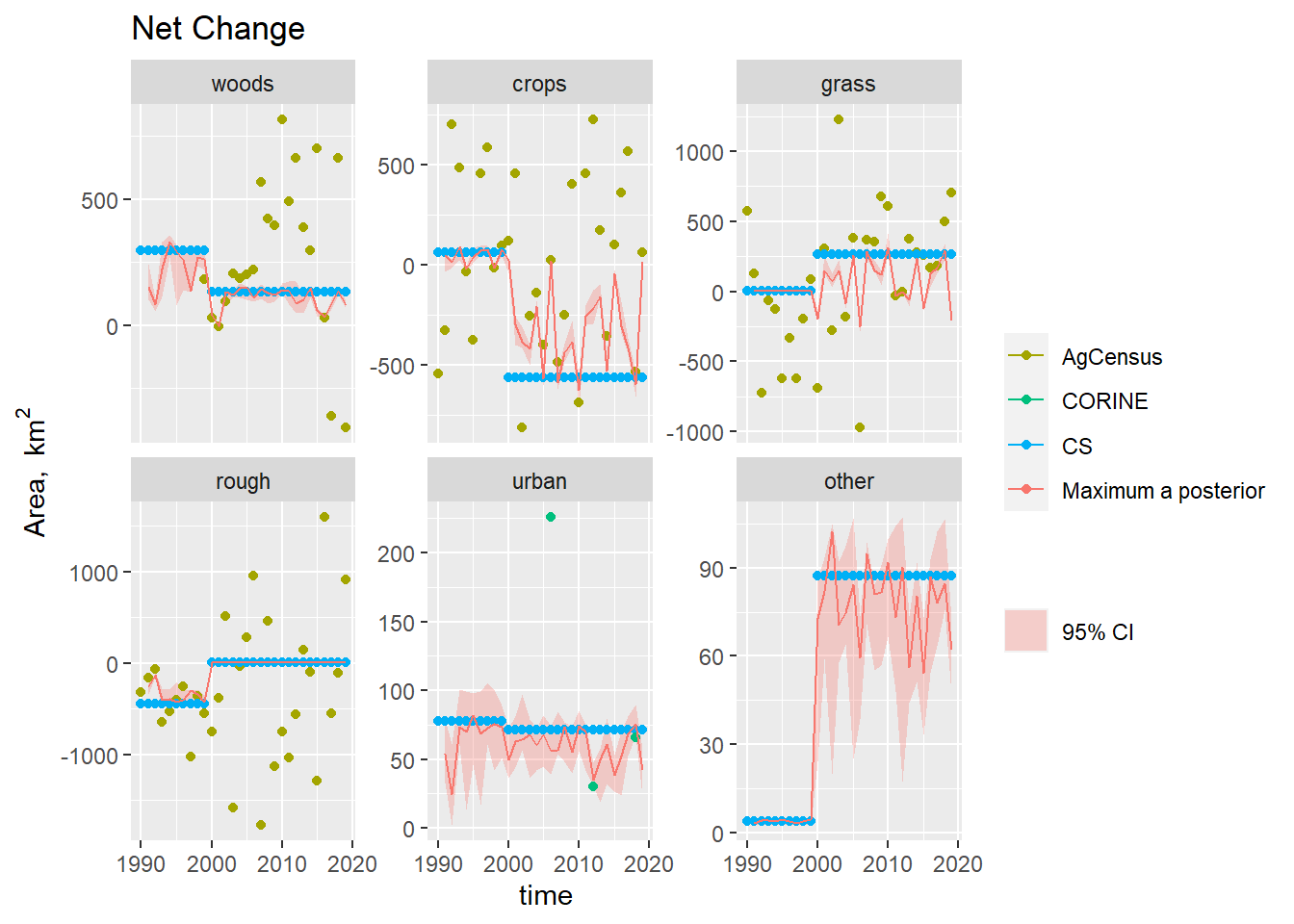
Figure 19.7: Time series of the net change in area occupied by each land use (\(\Delta A\)) from 1990 to 2019, showing the observations and posterior distribution of estimates. The shaded band shows the 2.5 and 97.5 % percentiles of the posterior distribution of the net change in area of each land use. The solid red line shows the maximum a posteriori prediction.
19.4 Discussion
In the current GHGI method, the CS and FC data are taken at face value as the estimate of land-use change. The results shown above represent an advance beyond this in several ways. Most obviously, the constraint of national-scale survey is introduced. This means that the \(B\) estimates are less subject to the sampling error associated with using only 544 sites across the UK. The Agricultural Census data is an imperfect constraint, as it specifies only net change, but it is based on a very comprehensive and long-standing census programme, and it far more likely to pick up the broad trends in national-scale land use over long periods of time. Secondly, our method quantifies uncertainty in a rigorous way, consistent with probability theory. This aspect could be improved by quantifying the uncertainty on the input observational data in a systematic way. Lastly, although we introduce only one additional data source beyond those used in the current GHGI to estimate \(B\), the framework is in place to introduce any other data sets we choose. For simplicity, we elected not to include the LCM, LCC, CORINE or IACS data in the results presented here. However, adding these in is a simple matter, if we choose to believe the observations or can improve their consistency.
References
Braak, Cajo J. F. ter, and Jasper A. Vrugt. 2008. “Differential Evolution Markov Chain with Snooker Updater and Fewer Chains.” Statistics and Computing 18 (4): 435–46. https://doi.org/10.1007/s11222-008-9104-9.
Hartig, Florian, Francesco Minunno, and Stefan Paul. 2017. “BayesianTools: General-Purpose MCMC and SMC Samplers and Tools for Bayesian Statistics.”
Levy, P., M. van Oijen, G. Buys, and S. Tomlinson. 2018. “Estimation of Gross Land-Use Change and Its Uncertainty Using a Bayesian Data Assimilation Approach.” Biogeosciences 15 (5): 1497–1513. https://doi.org/10.5194/bg-15-1497-2018.
Vrugt, Jasper A., James M. Hyman, Bruce A. Robinson, Dave Higdon, Cajo J. F. Ter Braak, and Cees G. H. Diks. 2008. “Accelerating Markov Chain Monte Carlo Simulation by Differential Evolution with Self-Adaptive Randomized Subspace Sampling.” International Journal of Nonlinear Sciences and Numerical Simulation, nos. LA-UR-08-07126; LA-UR-08-7126 (January). https://www.osti.gov/biblio/960766-accelerating-markov-chain-monte-carlo-simulation-differential-evolution-self-adaptive-randomized-subspace-sampling.