Section 20 Estimating Land-Use Change Spatially
20.1 Introduction
In the previous sections, we have estimated the posterior distribution of the \(B\) matrix for each year, using MCMC. Next, we need to use the \(B\) matrix to predict land-use change spatially. We do this by starting with the relatively well-known state of land use \(U\) at the present-day, and move backwards in time. At each time step, the \(B\) matrix for that year tells us how many grid cells need to change from each class to every other class. For a given element \(B_{ij}\) in the matrix, the candidate cells for change are all those where \(u = i\). We do not know exactly which cells actually changed in a given year, but there are several spatio-temporal data sets which gives us information about this. For example, LCC and IACS both have spatio-temporal observations of the time and location of agricultural land use. The Agricultural Holdings data tell us where and when the changes in crop, grass and rough grazing occurred, based on farmer census returns. The FC NFI/SCDB data tell us the location and planting dates of forestry. None of these data sets are perfect, and we may not believe the absolute magnitudes of change implied, but they tell us something about the probability of land being used for a given purpose at a given location and time. Our approach attempts to make the best use of the available data to estimate the location of each land-use change probabilistically. Again we use a Bayesian approach.
Each year, our aim is to sample from the posterior distribution of the land-use map \(U_{t-1}\). Because we have already established the \(B\) matrix, and we can consider each change to be independent, the problem is simply to choose the location of each change in accordance with Bayes Theorem. To do this, we can use a method referred to as “importance sampling” (Hartig et al. 2011). Importance sampling is a very efficient form of rejection sampling (aka the “accept-reject” algorithm, or Sequential Monte-Carlo (SMC)). In the previous section we used MCMC to sample from the posterior distribution. This is usually necessary, because we have to to evaluate the likelihood function across a wide range of high-dimensional parameter space by iterative numerical sampling. However, in the case of estimating the land-use map \(U_{t-1}\), the form of the model and the likelihood is so simple that we can calculate the likelihood in advance. The model is simply the identity function, and there are only six possible states {woods, crops, grass, rough, urban, other}. For each of these possible states, we can evaluate the likelihood \(\mathcal{L}\), the probability that the proposed land-use state \(\hat{u}\) is correct, given a vector of observations \(\textbf{u}\). For example, with a vector of observations \(\textbf{u}\) = {crop, crop, grass} from three data sources (e.g. LCM, IACS and CORINE), we might estimate the probability that the true land-use state is “crop” to be 2/3. If we know the precision of these data sources, we can adjust this accordingly. Similarily, if we have different observations, such as the probability of an increase in crop area in the local region, we can incorporate these also.
Having established these six likelihoods at each location for each year, we can then use these in the sampling process when choosing from the candidate cells for land-use change.
The basis of all sampling algorithms is that the probability of a parameter set belonging to the posterior distribution is proportional to the likelihood.
The simplest such algorithm, rejection sampling, works by choosing a huge number of possible parameter sets at random, often from a uniform distribution; the chance of their being accepted is proportional to their likelihood.
Importance sampling is similar, but the candidates are sampled with some importance weighting, such that they are somehow sampled approximately in proportion to their likelihood. The inefficient rejection step can be minimised because improbable parameters sets are not being selected in the first place.
Here, we have the extreme case where we exactly know the likelihood in advance, so can use this in weighting the sampling process such that all samples can be ascribed to the posterior distribution.
We use the sampling algorithm in the R package wrswoR to implement this.
20.2 Methods
The implementation of importance sampling described above breaks down into a number of tasks.
Firstly, we evaluate the likelihood function for each of the six possible states {woods, crops, grass, rough, urban, other} for all years and at all locations. Computing this for 30 years at a resolution of 100 m requires ~two hours and a large amount of memory, but is feasible on JASMIN, and considerable stream-lining is possible in future.
Then, we begin with the present-day land-use map \(U_{t}\), as defined by LCM in 2019, with additional forest where this is reported in the current FC NFI/SCDB or FSNI data. This is a 100-m resolution raster grid, with 91 million cells, of which ~24 million of which are on land. For each year from the present-day going backwards:
- select a \(B\) matrix from the 2000 posterior samples produced in the [previous section][Data Assimilation: Estimating \(B\) by MCMC];
- for each element \(B_{ij}\), define the candidate cells as those where \(u = i\);
- select the number of cells specified by \(B_{ij}\) from the set of candidate cells, with the probability of inclusion being proportional to \(\mathcal{L}_{u=j}\);
- for the selected cells, set the new land use to equal \(j\).
- remove the selected cells from the candidate set so they cannot be resampled that year;
- when this has been completed for all elements \(B_{ij}\), move to the next year back in time and repeat until the starting year is reached (1990 in this case).
The above procedure produces a single sample from the posterior distribution of \(\mathbf{U}\), and it can be repeated to produce as many samples as desired. How many many samples are required will depend on the purpose at hand.
The basics of this procedure are very simple, and it can be repeated there is no good model for predicting which cells change in any given year. Having \(B_{ij}\) matrix, the candidate cells for change are all those where \(u = i\). the state of land use \(U\) at the next time step. Although there are predictable patterns in which cells tend to be used for forest, crops or grassland etc., exactly when a given cell will change land use is not predictable; the process is effectively stochastic for our purposes.
20.3 Results
All the maps here show 1-km resolution data because higher resolution is not easily discernible for large areas on typical graphical devices. However, all these data are originally produced at 100-m, and aggregated to lower resolution for display and summary purposes. The plots below show maps of the likelihood \(\mathcal{L}\) for each of the six land uses (Figures 21.1-21.6). These show little that is unexpected. The likelihood is expressing the number of data sources which predict that land-use type, as a fraction of the number of data sources available. It thereby effectively averaging predictions of that land-use type across the data sources. The likelihood of the presence of woods is dominated by the FC NFI/SCDB data, so the maps closely resemble this, but with the addition of other data sources which include the location of woods (LCM, CORINE, and IACS). The likelihood of the presence of crops is an amalgamation of all the data sources which include the location of crops (LCM, LCC, CORINE, IACS, Agricultural Holdings). The same principles apply to the other land-use types.
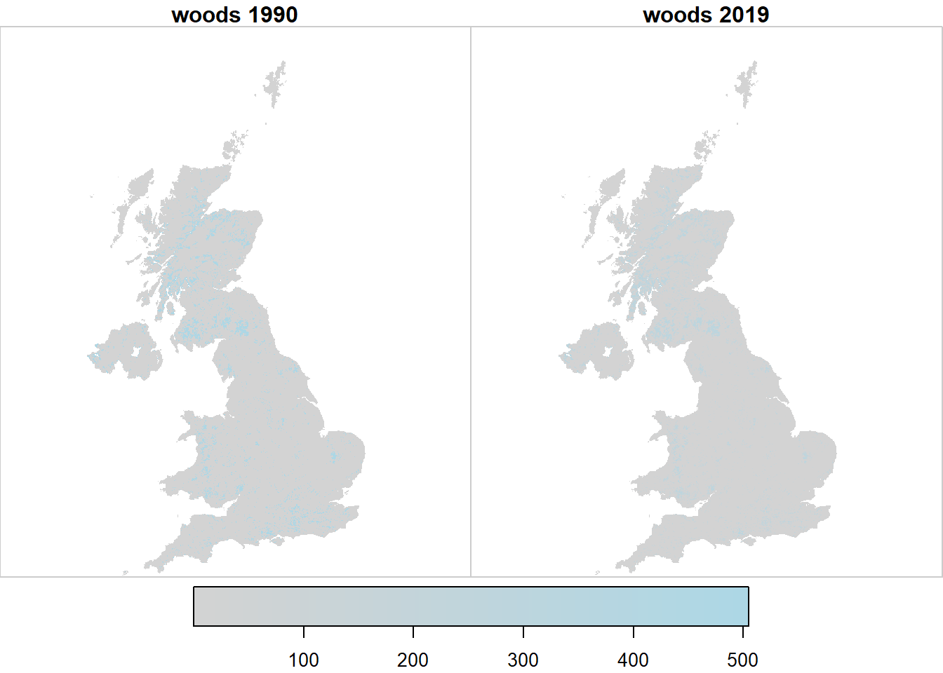
Figure 20.1: Spatial variation in the likelihood \(\mathcal{L}\) of observing land use \(u\) at two example points in time, arbitrarily rescaled for plotting.
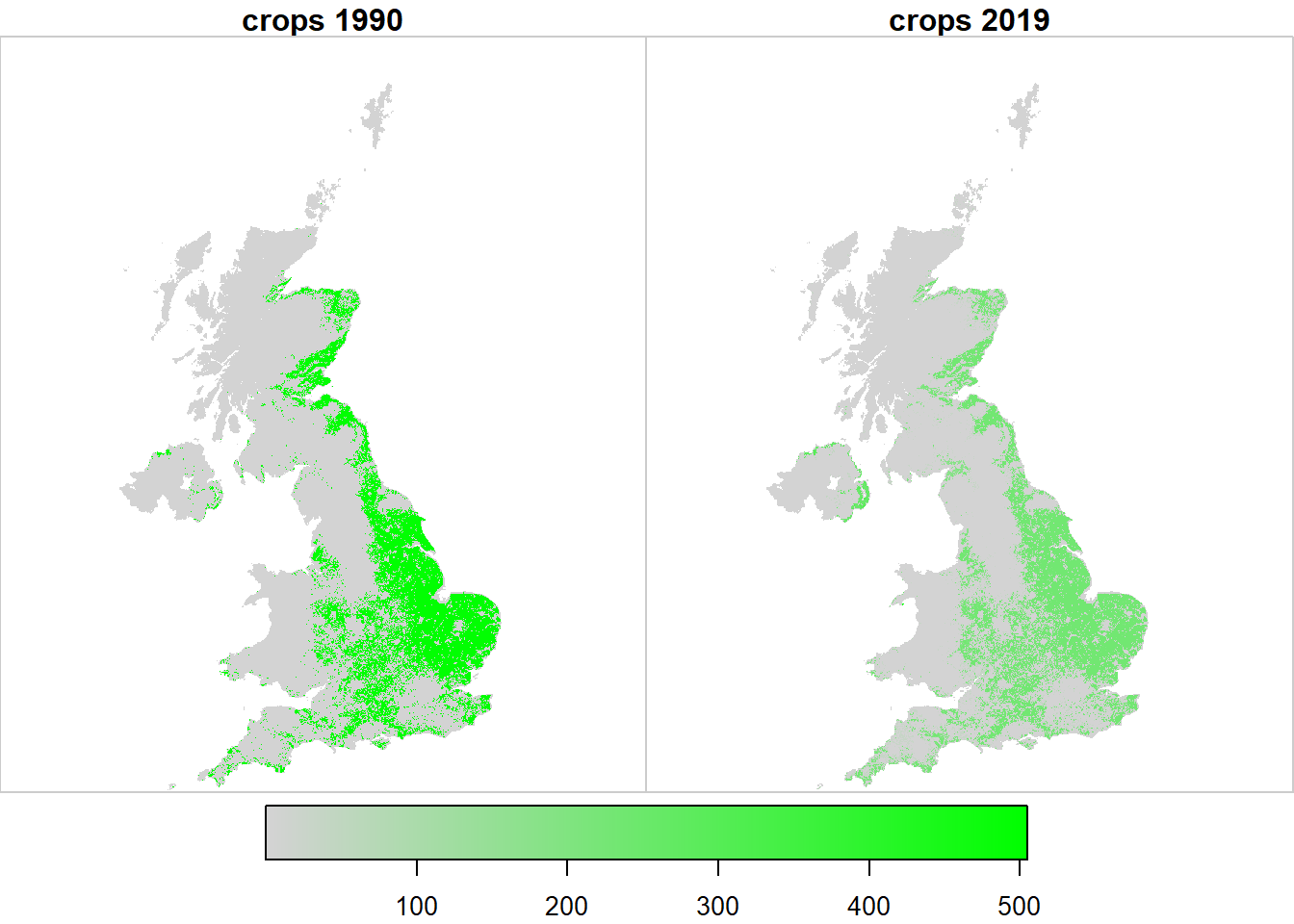
Figure 20.2: Spatial variation in the likelihood \(\mathcal{L}\) of observing land use \(u\) at two example points in time, arbitrarily rescaled for plotting.
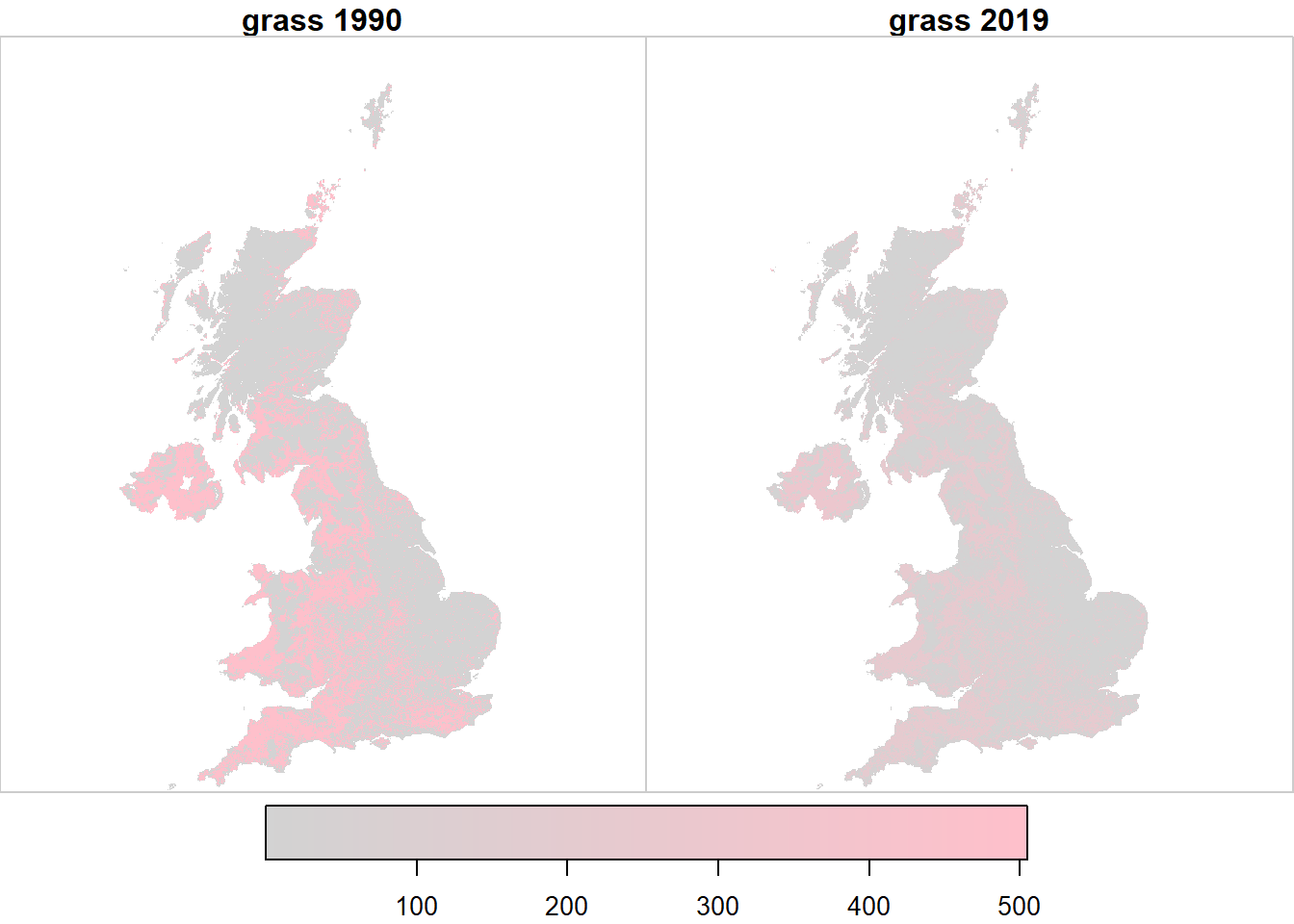
Figure 20.3: Spatial variation in the likelihood \(\mathcal{L}\) of observing land use \(u\) at two example points in time, arbitrarily rescaled for plotting.
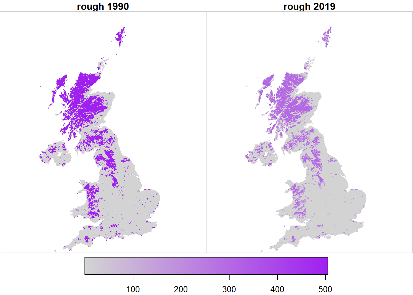
Figure 20.4: Spatial variation in the likelihood \(\mathcal{L}\) of observing land use \(u\) at two example points in time, arbitrarily rescaled for plotting.
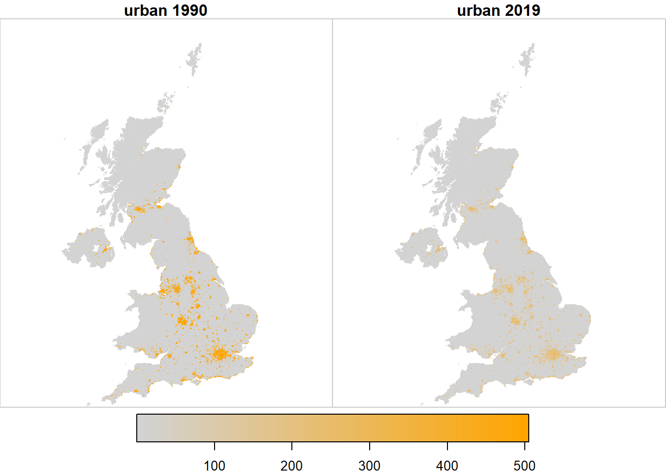
Figure 20.5: Spatial variation in the likelihood \(\mathcal{L}\) of observing land use \(u\) at two example points in time, arbitrarily rescaled for plotting.
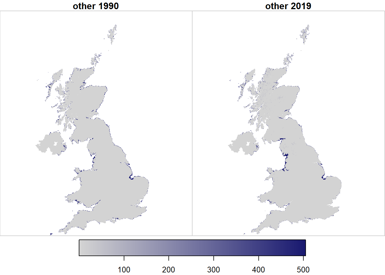
Figure 20.6: Spatial variation in the likelihood \(\mathcal{L}\) of observing land use \(u\) at two example points in time, arbitrarily rescaled for plotting.
Figure 20.7 shows the outcome from the importance sampling algorithm described in the Methods. The 2019 map is defined solely by observations (LCM, FC NHI/SCDB, and FSNI data). The 1990 map is the result of applying the set of land-use changes prescribed in the series of annual \(B\) matrices from the posterior distribution. This map is thus based on the magnitude and nature of land-use change from the data sources in which we have highest confidence in their consistency over time (CS, FC and AgCensus), and applies this spatially, using the data sources which provide information on the spatial pattern of land use change. Because the absolute extent of land changing use is small, and it tends to occur with relatively small granularity. Differences are not easily apparent when viewing the whole UK, or even at a Devolved Administration level (Figures 20.8, 20.9, 20.10), but we show these here for completeness.
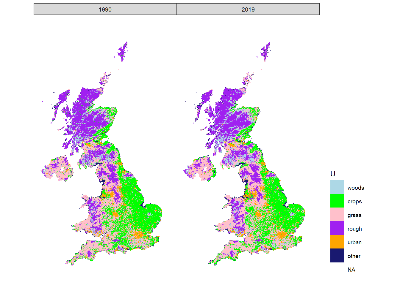
Figure 20.7: Estimated state of land-use \(U\) in 1990 and 2019 in the UK.
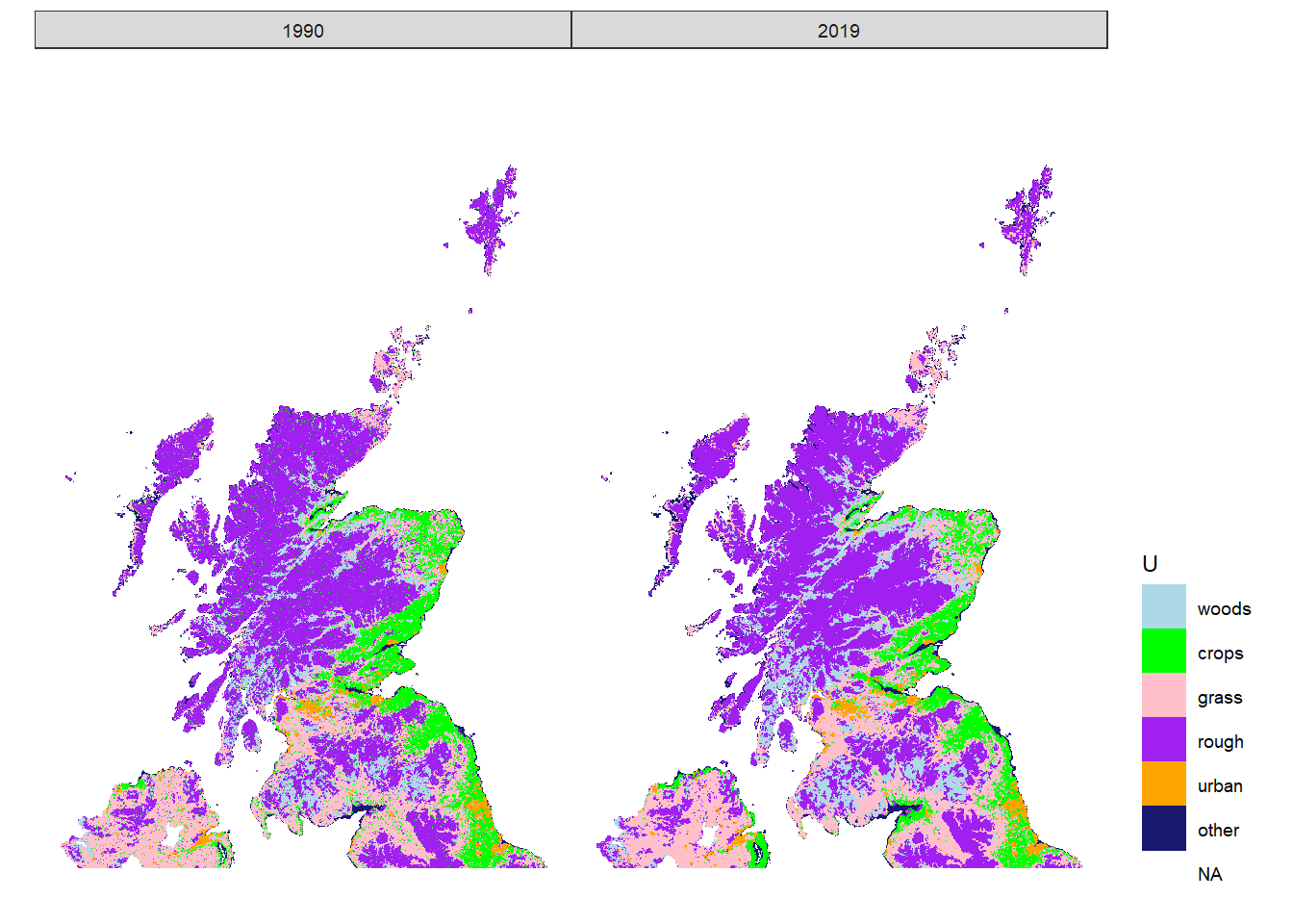
Figure 20.8: Estimated state of land-use \(U\) in 1990 and 2019 in Scotland and Northern Ireland.
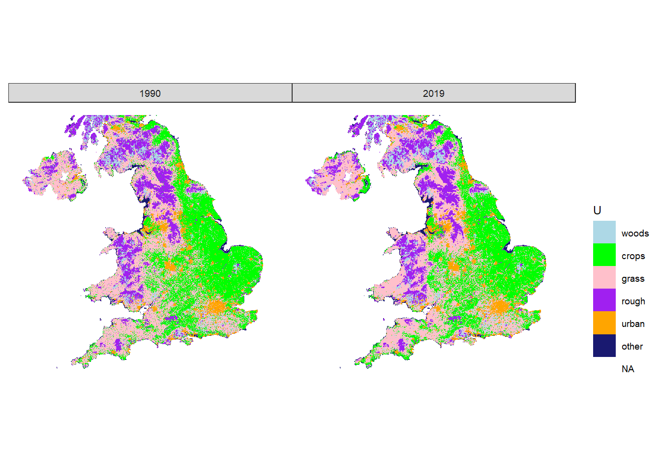
Figure 20.9: Estimated state of land-use \(U\) in 1990 and 2019 in England.
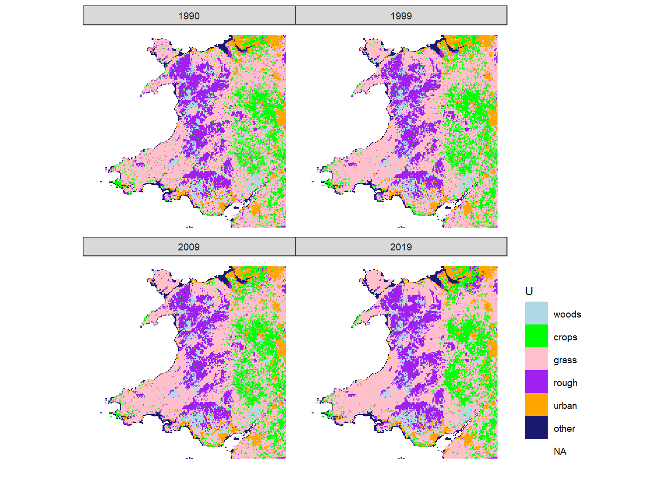
Figure 20.10: Estimated state of land-use \(U\) in 1990, 1999, 2009 and 2019 in Wales.
Slightly more useful is to zoom in on smaller regions. Figures 20.11 and 20.12 show two 100 x 100 km regions in Scotland, to illustrate the potential for analysing these results in by comparison with other mapped data. The broad expected patterns, such as some areas with known urbanisation over this period can be identified. However, beyond basic sense-checking, a detailed spatio-temporal analysis of this output has not yet been done.
For the purposes of the UK GHGI, the actual spatial patterns are not important in themselves (although obviously desirable). As currently implemented, there are no explicitly spatial terms in the soil carbon modelling. Instead, we can summarise the spatio-temporal data cube \(\mathbf{U}\) as the set of unique vectors of land use. To greatly reduce the volume of input and output data, the soil carbon model can be applied to this much smaller set of inputs. We analyse the output of the data assimilation procedure in terms of these vectors in the next section.
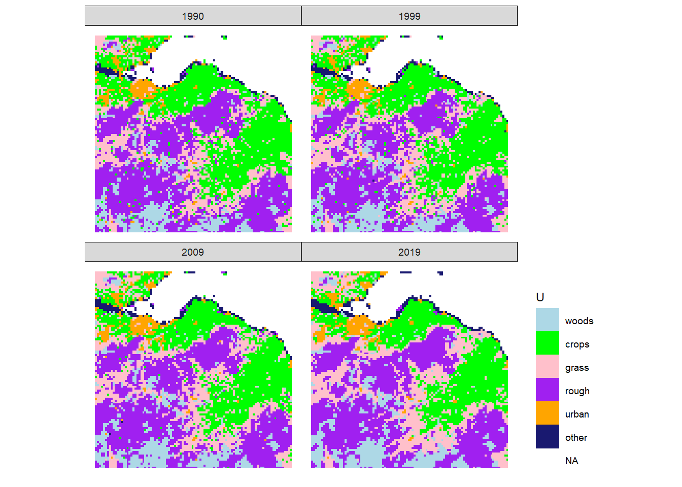
Figure 20.11: Estimated state of land-use \(U\) in 1990, 1999, 2009 and 2019 in the 100 x 100 km square containing Edinburgh.
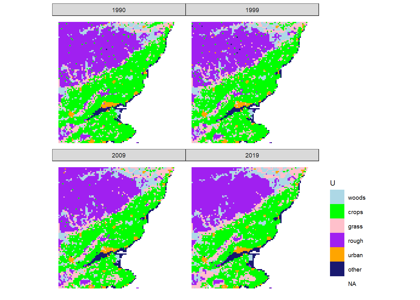
Figure 20.12: Estimated state of land-use \(U\) in 1990, 1999, 2009 and 2019 in the 100 x 100 km square centred on Dundee.
Figures 20.13, 20.14 and 20.15 show the results in the form of the vectors with greatest area (most frequent).
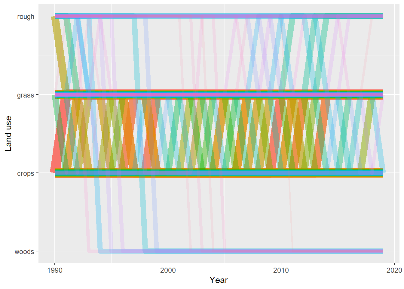
Figure 20.13: Trajectories of the 100 land-use vectors in the posterior \(U\) with the largest areas (excluding the six vectors which show no change). Each vector of land use is shown in a different colour, varied arbitrarily to differentiate different vectors. Line thickness and opacity are proportional to the frequency of (or total area occupied by) each vector, so that the dominant vectors are the most visually obvious.
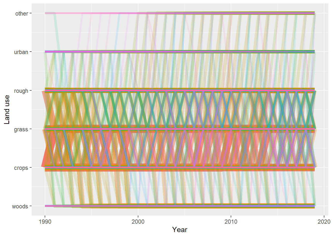
Figure 20.14: Trajectories of the 1000 land-use vectors in the posterior \(U\) with the largest areas (excluding the six vectors which show no change). Each vector of land use is shown in a different colour, varied arbitrarily to differentiate different vectors. Line thickness and opacity are proportional to the frequency of (or total area occupied by) each vector, so that the dominant vectors are the most visually obvious.
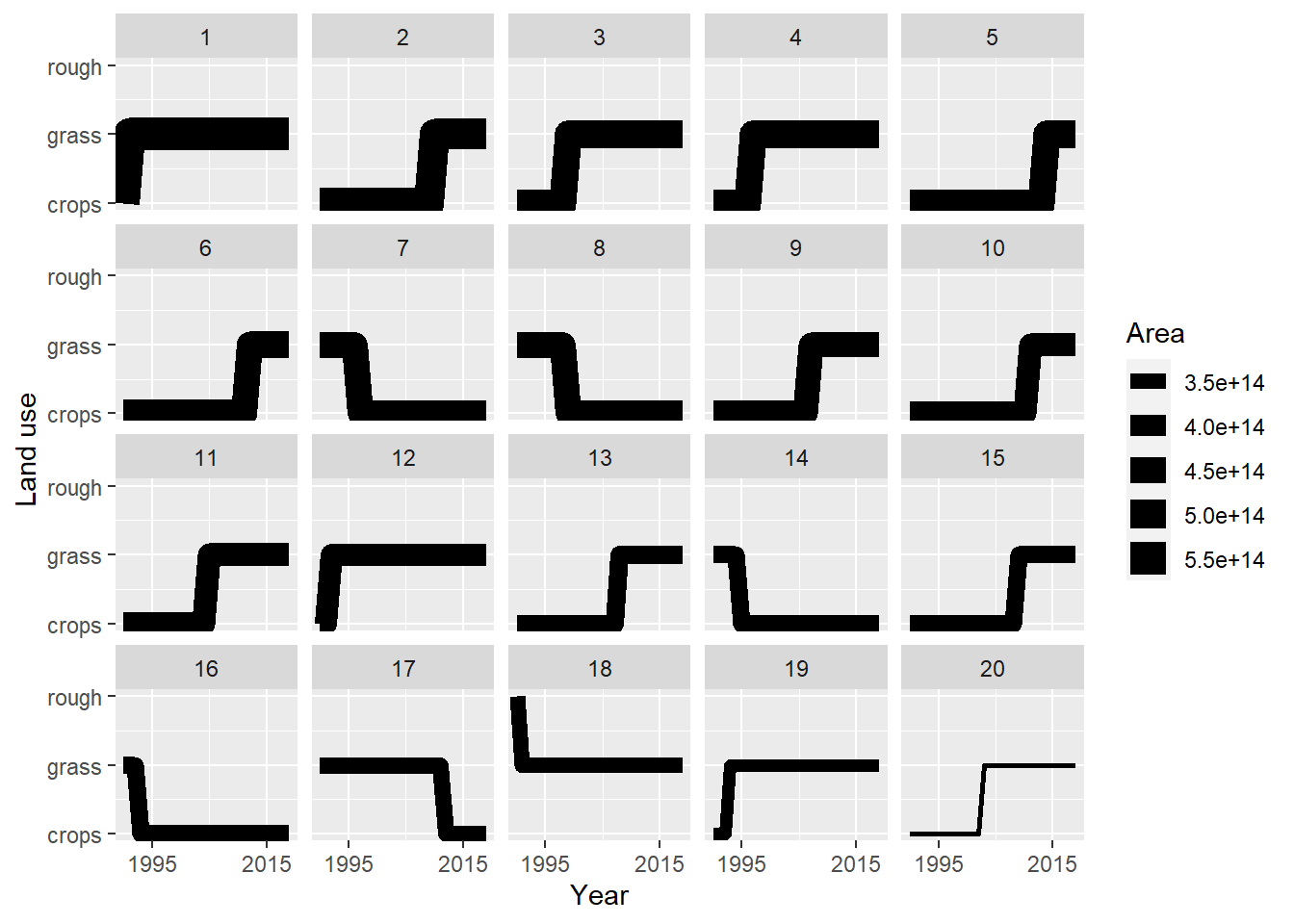
Figure 20.15: Trajectories of the 20 land-use vectors in the posterior \(U\) with the largest areas (excluding the six vectors which show no change). Line thickness is proportional to the frequency of (or total area occupied by) the vector
20.4 Discussion
Despite reducing the dimensions, the land-use vectors are still a high-dimensional structure to visualise. The plots in Figures 20.13, 20.14 and 20.15 show two ways to visualise the data. Attempts to make visualisation easier generally comes at the cost of presenting only a restricted amount of the total information. Some time exploring other methods for visualisation would be worthwhile. The figures show that the dominant vectors contain the transitions between crop & grass and vice versa. There are no rotational changes in the top 20 vectors (Figure 20.15) i.e. involving changes back and forth at the same location. The frequency of such changes, and whether this matches expectations, remains to be examined. Figures 20.13, 20.14 and 20.15 show only a single set of vectors, based on the MAP \(B\) matrix. In fact, we have 2000 samples from the whole distribution, but showing the uncertainty in data like this, with categorical and continuous features, is particularly difficult.
References
Hartig, Florian, Justin M. Calabrese, Björn Reineking, Thorsten Wiegand, and Andreas Huth. 2011. “Statistical Inference for Stochastic Simulation Models – Theory and Application.” Ecology Letters 14 (8): 816–27. https://doi.org/10.1111/j.1461-0248.2011.01640.x.