Section 18 Estimating \(B\) by Least-Squares Optimisation
18.1 Introduction
As a first step in the data assimilation (DA) procedure, we show that it can be done in a relatively simple way. In this section, we use a least-squares (LS) optimisation algorithm to estimate the \(B\) matrix parameters. This is done for a number of reasons.
- Firstly, for the purposes of elucidation, we show that the DA procedure can be separated from the Bayesian aspect.
- Secondly, there is also a practical reason: when estimating the \(B\) parameters by MCMC in the following section, it is helpful to have an idea of sensible starting values. MCMC chains can be initialised with entirely random values, but starting at least one chain in a region of high posterior probability speeds up the process considerably.
- Lastly, by doing the DA in a non-Bayesian way, we can illustrate the advantages of the Bayesian approach.
18.2 Methods
Firstly, we define a function to calculate the root-mean-square error (RMSE) for a given \(B\) matrix. RMSE is commonly used as a measure of the differences between observed values and those predicted by a model. Here, we have observations of land-use change in the form of \(\Delta A, G, L\) and \(B\) observed by several different data sources. For comparison, we have the given \(B\) matrix and the resulting predictions of \(\Delta A, G\) and \(L\) that this produces via the equations in Methods. The difference between the observations and predictions gives the residual; for each term \(\Delta A, G, L, B\) this is squared, averaged, and the square root taken to give the RMSE. Because all terms have the same dimensions (km2 / year), we can simply add them. There are various permutations on the exact way in which the RMSE could be calculated here, but this is sufficient for our purposes. There are numerous optimisation algorithms, which will vary parameters iteratively to minimise a function. Here we use the algorithm of Byrd et al. (1995). For each year between 1990 and 2019, we run this algorithm to find the \(B\) matrix parameter set which has the smallest RMSE value, i.e. parameter set which best fits to the observed data.
18.3 Results
The figures below (18.1, 18.2, 18.3, and 18.4) show the same observed data as in the previous section, with the addition of the estimates from least-squares optimisation (black solid line). The least-squares fit is largely as expected, fitting through the centre of the observations, and following the same trends. Each of the terms \(\Delta A, G, L\) and \(B\) are given equal weighting, and within these, all of the observations are given equal weighting.
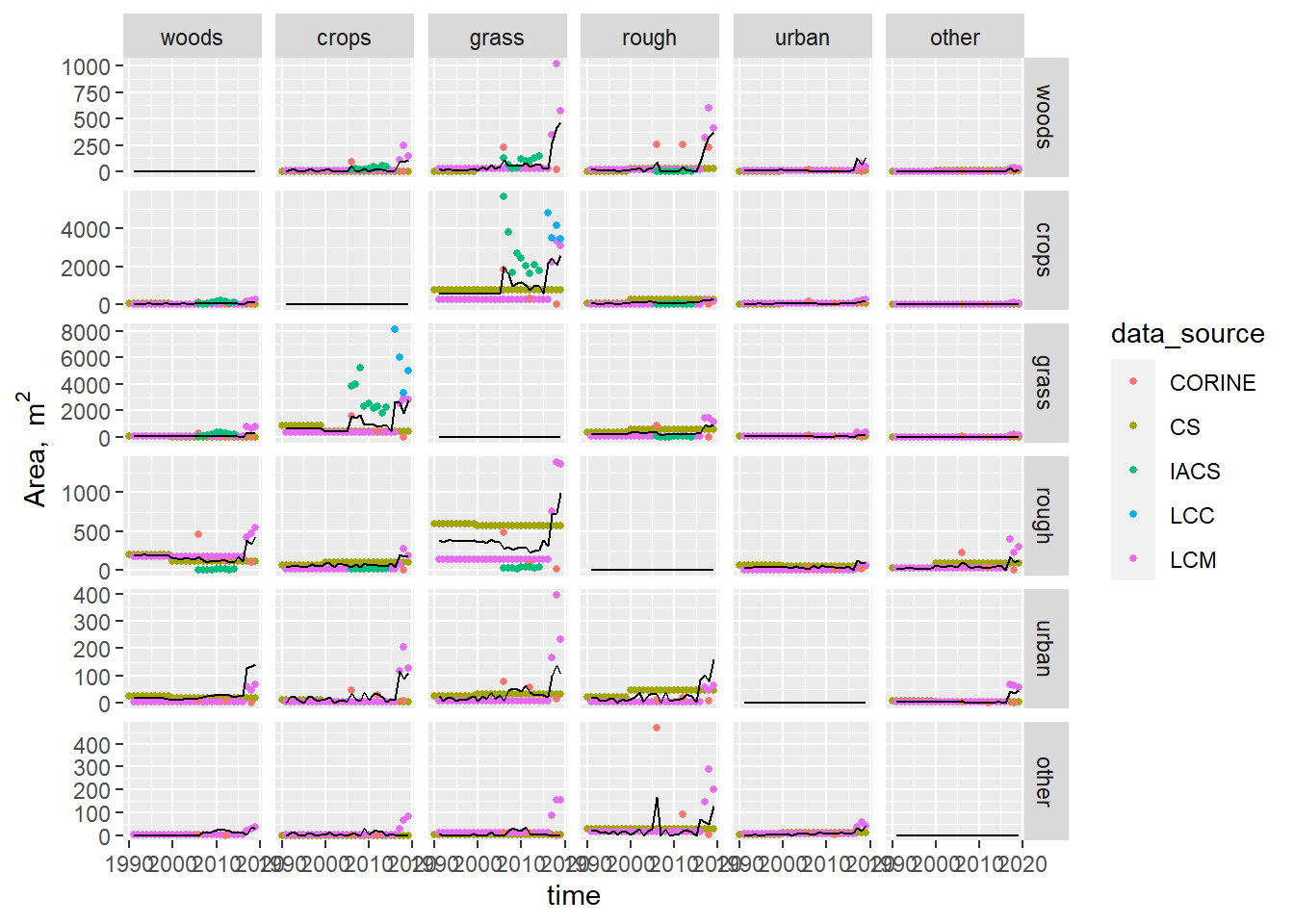
Figure 18.1: Time series of area changing from each land use to every other land use (the matrix \(\mathbf{B}\)) observed by different data sources. Coloured symbols show the observations; the black line shows the best-fit values estimated by least-square optimisation. LCM and CS values between surveys were interpolated values as constant annual rates.
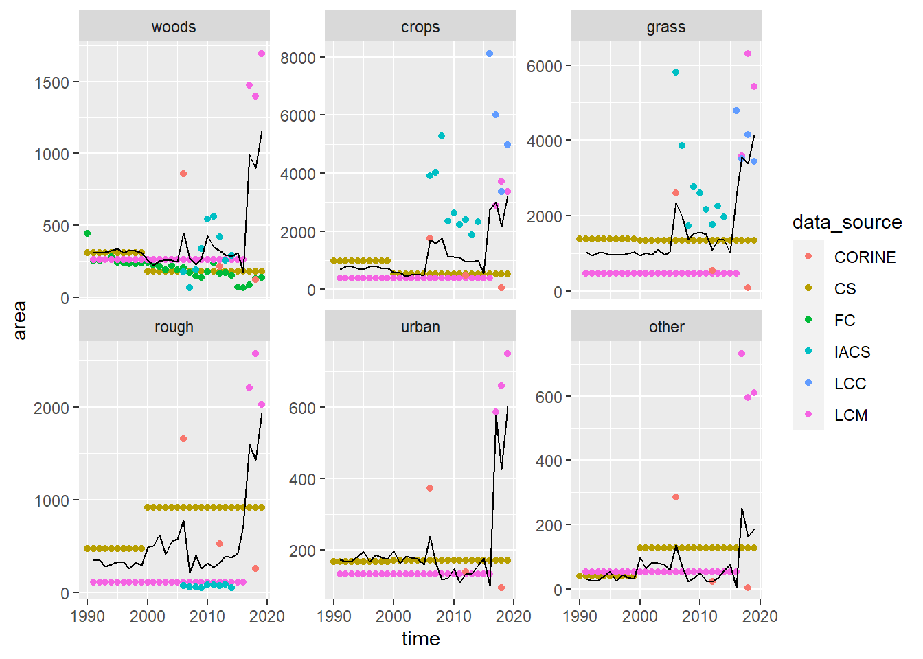
Figure 18.2: Time series of gross gain in area \(\mathbf{G}\) of each land use observed by different data sources. Coloured symbols show the observations; the black line shows the best-fit values estimated by least-square optimisation. LCM and CS values between surveys were interpolated values as constant annual rates.
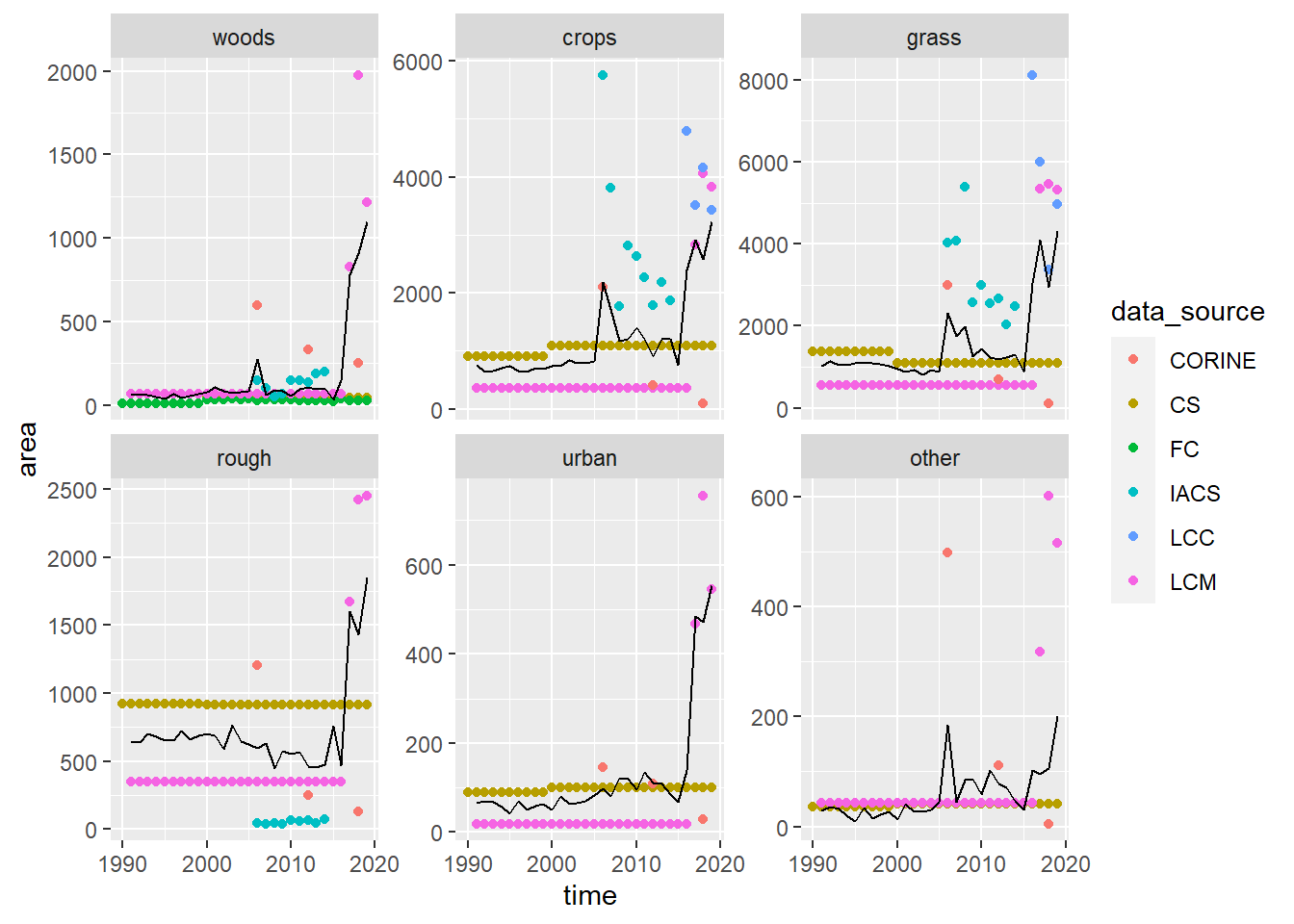
Figure 18.3: Time series of gross losses of area \(\mathbf{L}\) from each land use observed by different data sources. Coloured symbols show the observations; the black line shows the best-fit values estimated by least-square optimisation. LCM and CS values between surveys were interpolated values as constant annual rates.
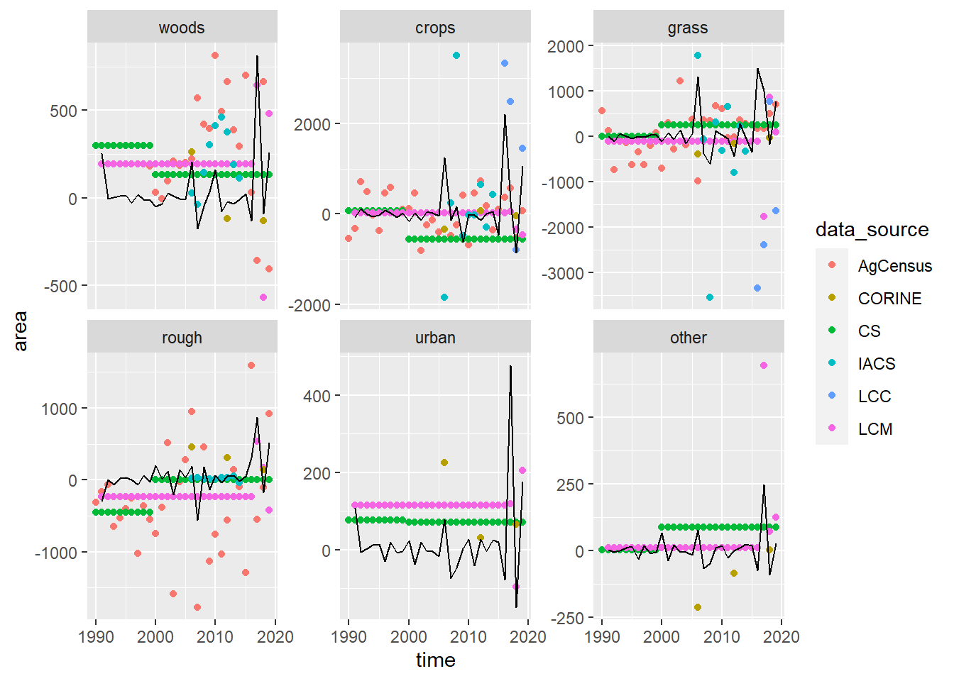
Figure 18.4: Time series of net change in area \(\Delta \mathbf{A}\) of each land use observed by different data sources. Coloured symbols show the observations; the black line shows the best-fit values estimated by least-square optimisation. LCM and CS values between surveys were interpolated values as constant annual rates.
18.4 Discussion
One purpose of the exercise is to show that the DA procedure can be done in a simpler, non-Bayesian way, and the figures above show that this is possible. The practical purpose, to provide a quick method to give initial values for MCMC chains is demonstrated by the results above.
More informatively, two main weaknesses of the non-Bayesian approach are apparent. Firstly, no quantification of uncertainty is provided. The LS algorithm identifies the single parameter set which has the best fit with the data, given our definition of RMSE. However, it gives us no estimate of the probability of any other parameter set, nor does it tell us anything about the confidence we should have in predictions.
Secondly, our definition of RMSE is somewhat arbitrary. We implicitly assume that small RMSE values relate to high likelihoods, and that our best-fit parameter set might approximate to that with the maximum likelihood. However, we have not explicitly calculated the likelihood. Where this really matters is if we want to make the likelihood function more complex, to allow us to combine data sources with different dimensions and degrees of uncertainty. We implicitly give each observation the same uncertainty, and we can only add up the different terms in our RMSE because they happen to have the same units. If either of these were not the case, we could attempt to add in some arbitrary weightings to address this. However, the Bayesian approach explicitly calculates the likelihood, which is the probabilistically-correct formulation of the problem. In the present context, it is the answer to the question “what is the probability of observing the data if we know \(B\)?” (Oijen 2020). For each observation, no matter what its source, measurement uncertainty or units, we obtain a probability, not an arbitrary residual. Because we are working in the common currency of probability, we can multiply the values for all observations to give the likelihood for the whole observation set - parameter set combination. This is the approach we apply in the next section.
References
Byrd, Richard H., Peihuang Lu, Jorge Nocedal, and Ciyou Zhu. 1995. “A Limited Memory Algorithm for Bound Constrained Optimization.” SIAM Journal on Scientific Computing 16 (5): 1190–1208. https://doi.org/10.1137/0916069.
Oijen, Marcel van. 2020. Bayesian Compendium. Springer International Publishing. https://doi.org/10.1007/978-3-030-55897-0.