Section 3 QA/QC Using Chess Data

3.1 Introduction

The game of chess provides a convenient analogue for land-use change. Because the system is small enough to count and visualise easily, and because we know the true state at all times, this is an ideal way to test our algorithms, providing quality assurance and quality control (QA/QC) for our code.

Chess is played on a 8 x 8 board, so a suitably small domain of 64 squares. We can consider the chess board to have three states analagous to land uses: occupied by either white pieces or black pieces, or empty. Mathematically, $u = \mathbf{white, empty, black}$. At the start, there are two rows occupied by white, two rows occupied by black, and four empty rows ($A_{\mathrm{white}} = 16, A_{\mathrm{black}} = 16, A_{\mathrm{empty}} = 32$. At each move by white, one piece is moved, so its origin square changes from white to empty, and its new square changes either from empty to white, or from black to white (if an opposing piece is taken). So for example, after the first move by each side, we have a $\mathbf{B}$ matrix:

##       white empty black
## white    15     1     0
## empty     1    30     1
## black     0     1    15

As the game proceeds and pieces are captured, the numbers of white and black cells decrease ($A_\mathrm{white}$ and $A_\mathrm{black}$) and the number of empty cells ($A_\mathrm{empty}$) increases. The starting position is always the same, so there are predictable spatial patterns in where each state is likely to be found. Thousands of chess games are freely available online, and can be used as pseudo-data for showing how the data assimilation procedure works, and testing it with simple cases.

3.2 Examples

The plots below show some example analyses which test the functions for (i) the calculation of the $\mathbf{B}$ matrix from the time series of spatial maps (or board states) $\mathbf{U}$ and (ii) the calculation of the time series of area $\mathbf{A}$, and the gross gains and losses $\mathbf{G}$ and $\mathbf{L}$, from the $\mathbf{B}$ matrix.

Here we use a single game of chess to provide the true course of land-use change over 83 years (moves). To simplify, we restrict this to the states at $t = (1, 11, 15, 80)$ years. If we designate this to be the true states, we can simulate two sets of observations with noise by selecting different time slices, in this case $t = (1, 3, 13, 60)$ and $t = (1, 12, 45, 83)$. This simulates data sets which are related to the true state, but differ because of measurement error. These $\mathbf{U}$ states are plotted below.

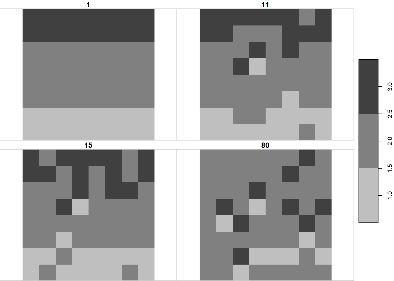
$True state of land use $\mathbf{U}$ at four time points, based on chess data.$

Figure 3.1: True state of land use $\mathbf{U}$ at four time points, based on chess data.

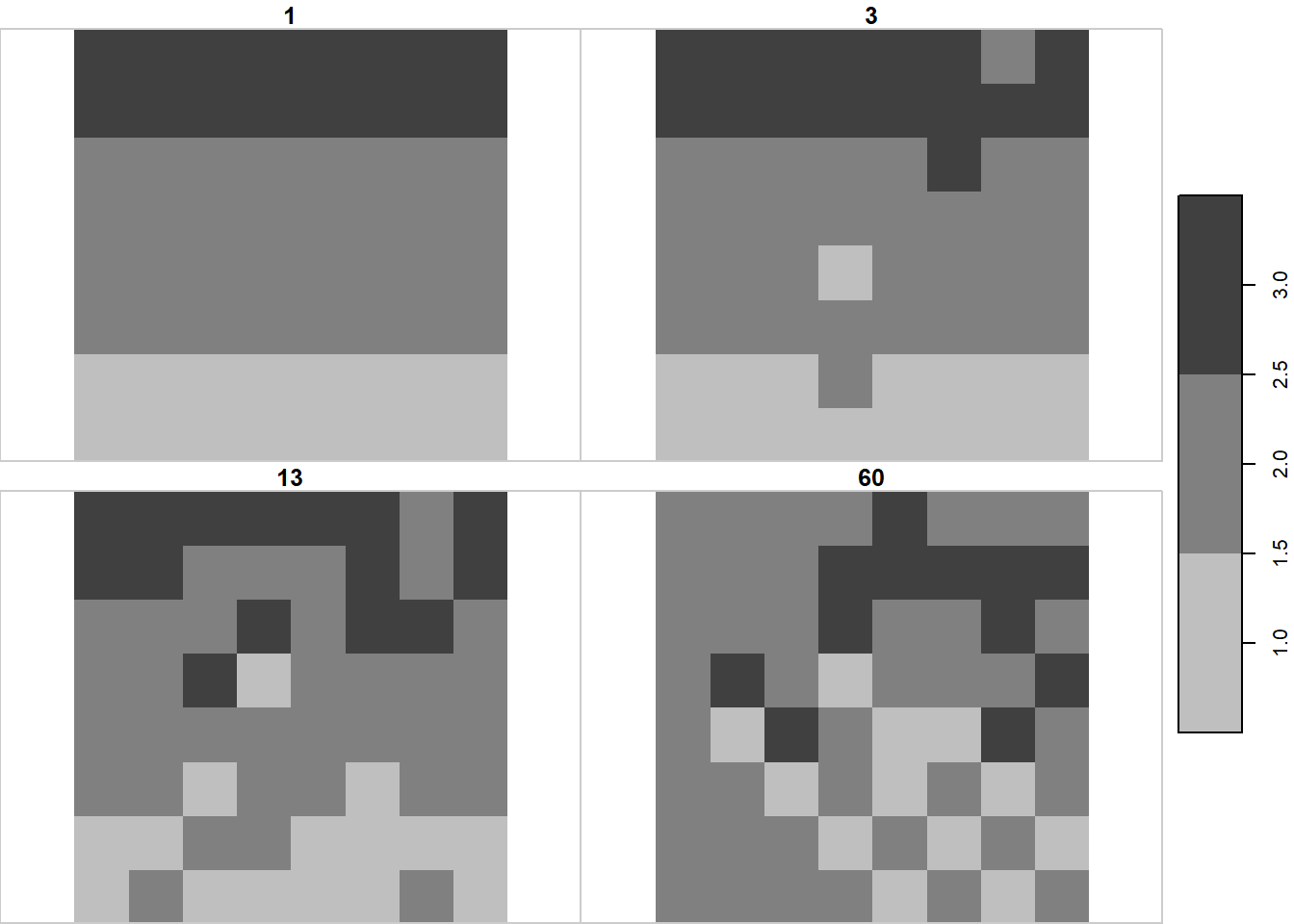
$Simulated observations of land use $\mathbf{U}$ at four time points, based on chess data, using time slices at different times from those designated as the true state. Denoted 'Obs1' in following figures.$

Figure 3.2: Simulated observations of land use $\mathbf{U}$ at four time points, based on chess data, using time slices at different times from those designated as the true state. Denoted ‘Obs1’ in following figures.

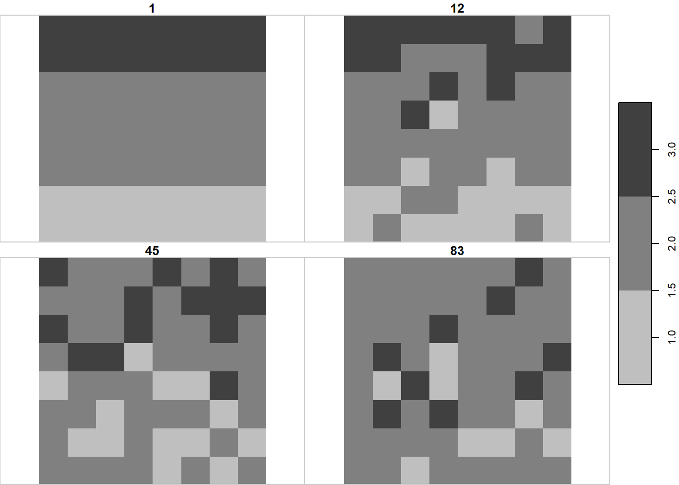
Figure 3.3: Simulated observations of land use $\mathbf{U}$ at four time points, based on chess data, using time slices at different times from those designated as the true state. Denoted ‘Obs2’ in following figures.

Subsequently, we have used these to test the performance of the data assimilation algorithm when confronted with imperfect data (results not shown). Here, we use these data as a basic QA/QC test, verifying that the functions correctly calculate the time series of $\mathbf{B}$, $\mathbf{A}$, $\mathbf{G}$, and $\mathbf{L}$. Verification is by simple cross-checking with the known values, which are easily calculated. The area of each cell is assumed to be 10 m^2 to provide a proper check on the consistency of units. The plots below show the time series of $\mathbf{B}$, $\mathbf{A}$, $\mathbf{G}$, and $\mathbf{L}$.

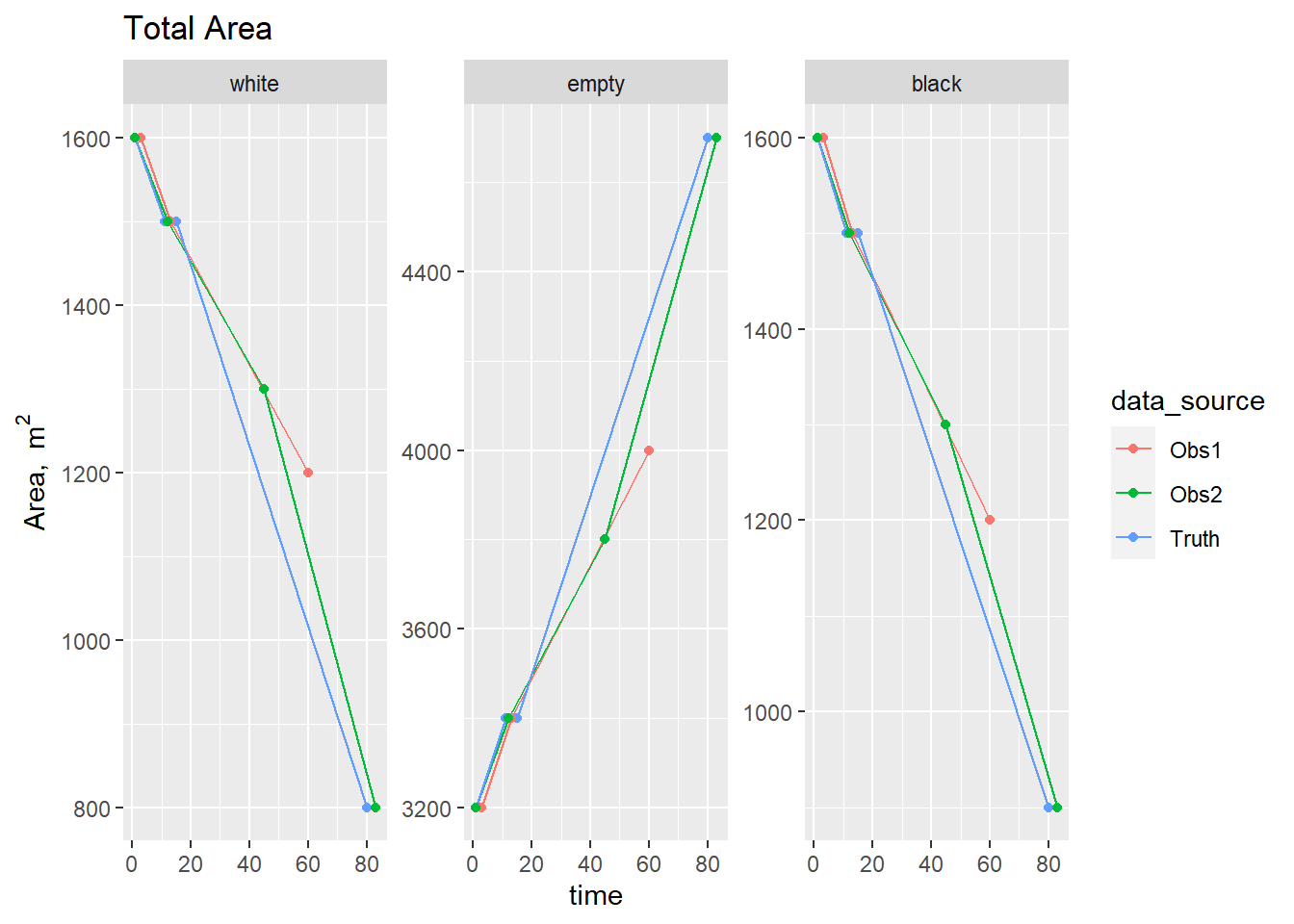
$Time series of area $\mathbf{A}$ from simulated data sources based on chess data.$

Figure 3.4: Time series of area $\mathbf{A}$ from simulated data sources based on chess data.

$Time series of area transitions $\mathbf{B}$ from simulated data sources based on chess data.$

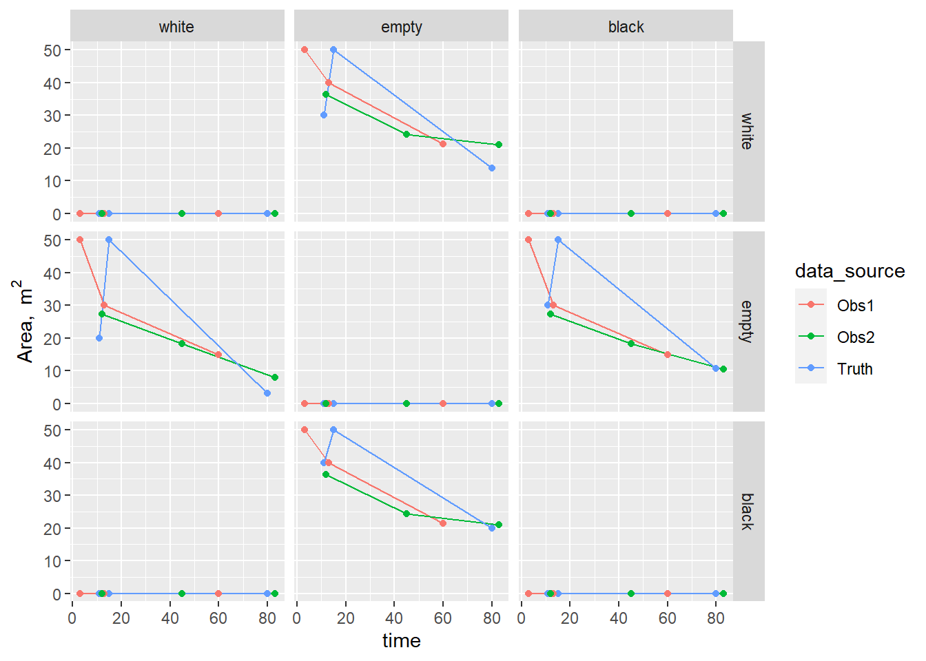
Figure 3.5: Time series of area transitions $\mathbf{B}$ from simulated data sources based on chess data.

$Time series of area gains $\mathbf{G}$ from simulated data sources based on chess data.$

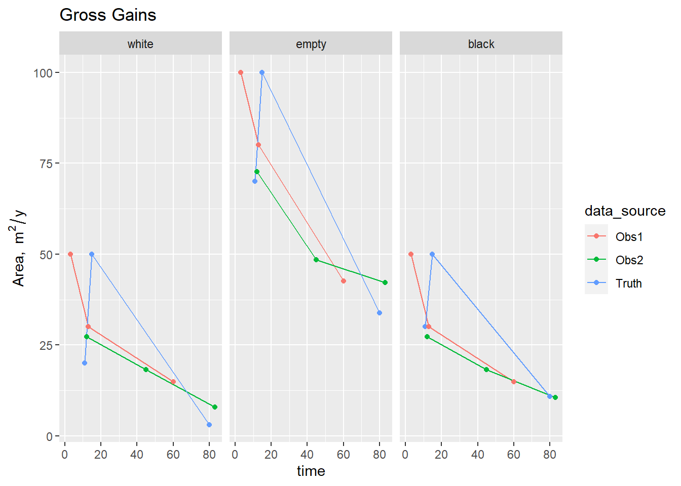
Figure 3.6: Time series of area gains $\mathbf{G}$ from simulated data sources based on chess data.

$Time series of area losses $\mathbf{L}$ from simulated data sources based on chess data.$

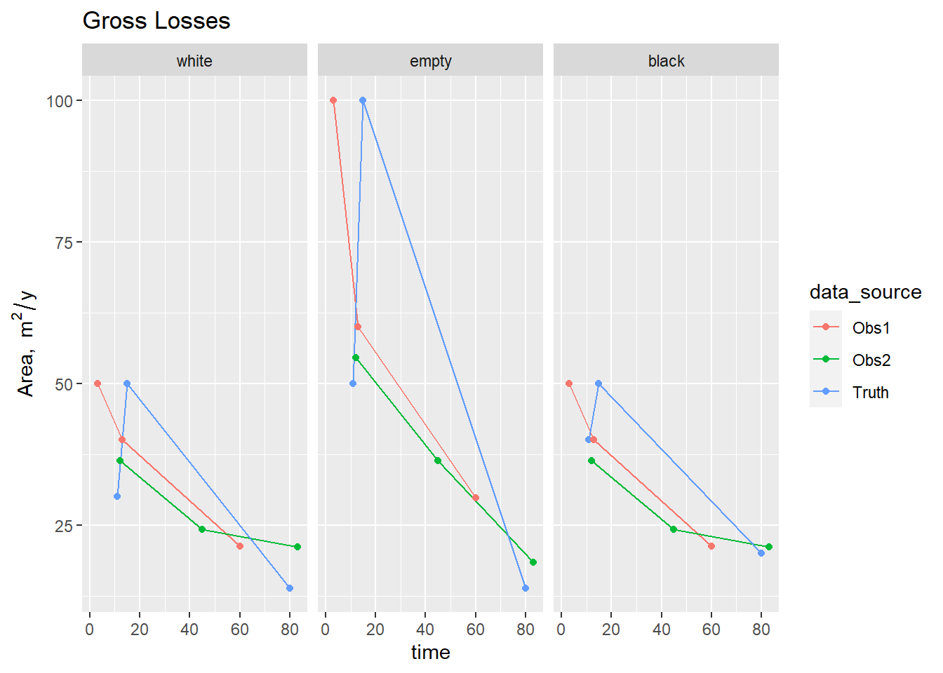
Figure 3.7: Time series of area losses $\mathbf{L}$ from simulated data sources based on chess data.